As you start reading about quantum mechanics, one of the first things you learn is that there are quantum jumps. But what the heck does that even mean? During quantum gates, for example, the wave function evolves continuously between the two qubit states. So in what sense is anything jumping?

The answer turns out to be surprisingly subtle - had I understood quantum jumps properly, I wouldn’t have been so puzzled about the mysterious qubit dynamics I raised in last week’s post. In today’s entry, I lay it out on the table to spare you from repeating my mistakes!

Watching a quantum jump

To understand quantum jumps, let’s consider a three-level system; for concreteness, I will use a simplified version of the calcium ion from the previous post. The qubit states are $\lvert 0\rangle =$ D_5/2 and $\lvert 1\rangle =$ S_1/2. We drive the transition between them with 729 nm light, and we measure the qubit by driving the S_1/2 ↔ P_1/2 transition with 397 nm light and collecting the fluorescence.

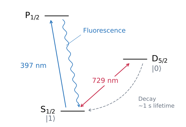
Three calcium-ion levels: qubit state 0 is D5/2 and state 1 is S1/2. A 729 nm drive connects the qubit states. A 397 nm laser excites S1/2 to P1/2, which emits fluorescence on returning to S1/2. D5/2 decays slowly to S1/2 with a mean lifetime of about one second.

If the ion is in $\lvert 1\rangle$, it scatters photons: it is bright. If it is in $\lvert 0\rangle$, the 397 nm light cannot excite it: it is dark. In the actual calcium ion, an 866 nm repumper keeps the fluorescence cycle running; I’ve left that extra level out of the diagram.

Suppose we prepare the qubit in $\lvert 0\rangle$, turn off the 729 nm drive, and leave the fluorescence measurement on. The dark state then spontaneously decays back to $\lvert 1\rangle$, with a mean lifetime of about a second: a prototypical “quantum jump”.

Let’s look for this “jump” in a simulation. First, I use QuTiP’s master-equation solver. For simplicity, I use a two-level system and represent detected fluorescence with the effective collapse operator

\[C_{\mathrm{det}} = \sqrt{R_{\mathrm{det}}}\,\lvert 1\rangle\langle 1\rvert, \qquad R_{\mathrm{det}} = 10^4\,\mathrm{s}^{-1}.\]

This represents a detected photon from the fluorescence cycle, which leaves the ion in $\lvert 1\rangle$. When the ion is bright, the detector counts at a mean rate of 10 kHz:

import numpy as np
import qutip as qt

zero, one = qt.basis(2, 0), qt.basis(2, 1)  # D5/2, S1/2
bright = one.proj()
tau = 1.0             # mean D5/2 lifetime (s)
R_det = 10_000.0      # 10 kHz count rate
times = np.linspace(0, 5, 101)

c_ops = [
    np.sqrt(1 / tau) * one * zero.dag(),  # spontaneous D -> S decay
    np.sqrt(R_det) * bright,             # effective detected fluorescence
]
H = 0 * bright  # no coherent evolution, only decay and fluorescence

result = qt.mesolve(
    H, zero, times, c_ops, e_ops=[R_det * bright],
    options={"method": "diag"},
)
mean_rate = result.expect[0]

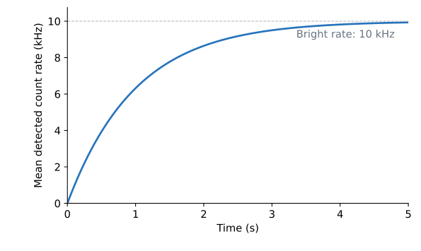
What we see is that the mean count rate rises smoothly toward 10 kHz, following an exponential: but where is my jump?

The master-equation mean detected count rate rises smoothly from zero toward 10 kHz, with a one-second exponential time constant. This is the average over repeated experiments.

The simulation above doesn’t show jumps because the master-equation solver evolves the average state over many repetitions. To simulate individual experiments, we can use QuTiP’s probabilistic quantum-trajectory solver to sample sequences of decay and fluorescence events:

bin_width = 0.05  # count photons in 50 ms bins
edges = np.linspace(0, 5, 101)
shots = qt.mcsolve(
    H, zero, edges, c_ops, ntraj=9, seeds=20260916,
    options={"progress_bar": "", "store_states": False, "method": "diag",
             "norm_t_tol": 1e-12, "norm_tol": 1e-6, "norm_steps": 100},
)

rates = []
for jump_times, channels in zip(shots.col_times, shots.col_which):
    detected = np.asarray(jump_times)[np.asarray(channels) == 1]
    counts, _ = np.histogram(detected, bins=edges)
    rates.append(counts / bin_width)

Here is what it gives:

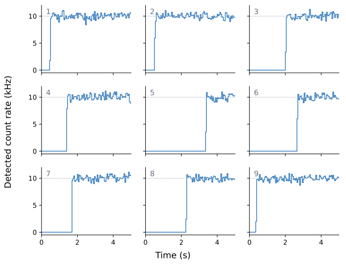
Nine simulated photon-count records. Each begins dark, then starts fluorescing at a different random time, with detected counts fluctuating around 10 kHz. Time runs from zero to five seconds in every panel.

What we find is that, in any individual experiment, the detector stays dark until the ion decays, at which point it abruptly starts counting at a constant mean rate of 10 kHz. The photon arrivals still fluctuate, but the signal switches from dark to bright rather than gradually increasing. This is the quantum jump we were looking for!

The paradox

So the question remains: how do we get the population into $\lvert 0\rangle$ in the first place?

You might think that, starting in $\lvert 1\rangle$, this requires the capacity to do an X gate on the qubit transition. But this is wrong!

It turns out that, in contrast to quantum gates, you can leave the qubit laser on continuously and see quantum jumps over a surprisingly broad range of powers and frequencies. This helps explain why directly driven quantum jumps were observed in trapped-ion systems almost a decade before the first trapped-ion quantum logic gates.

Why is that? What makes the qubit laser so effective?

The solution

It turns out that the physics is more nuanced than “one laser excites and another laser measures”. The sheer presence of the measurement laser, applied simultaneously with the qubit laser, changes how quickly population moves between the qubit states. The measurement laser can suppress or enhance transfer through what’s known as the quantum Zeno and anti-Zeno effects.

First, we can see this directly in a simulation of a three-level system, again using ⁴⁰Ca⁺ and the same 729 nm Rabi frequency as the last post. Here the 397 nm laser is resonant, and I approximate S–P as a closed fluorescence cycle, omitting Zeeman sublevels and the repumper. The P-state decay rate uses its measured lifetime:

D, S, P = [qt.basis(3, i) for i in range(3)]
Omega = 2 * np.pi * 162_806  # fitted value, approximately 2π × 163 kHz
Gamma = 1 / 6.904e-9         # P-state decay rate (1/s)
tau_D = 1.168               # D-state lifetime (s)

def population(detuning_hz, Omega_397, times):
    H = (-2 * np.pi * detuning_hz * D.proj()
         + Omega / 2 * (S * D.dag() + D * S.dag())
         + Omega_397 / 2 * (S * P.dag() + P * S.dag()))
    c_ops = [np.sqrt(Gamma) * S * P.dag(),
             np.sqrt(1 / tau_D) * S * D.dag()]
    result = qt.mesolve(
        H, S, times, c_ops, e_ops=[D.proj()],
        options={"method": "diag", "normalize_output": False},
    )
    return result.expect[0]

times = [np.linspace(0, 3.1e-6, 801), np.linspace(0, 80e-6, 8001)]
detunings = [0, 1e6]  # on resonance and 1 MHz detuning

First, as a sanity check, let’s see what happens when the measurement beam is off, setting $\Omega_{397}=0$:

without_measurement = [population(d, 0, t) for d, t in zip(detunings, times)]

On resonance, a π pulse transfers almost all the population to D. At 1 MHz detuning, the population oscillates but never exceeds about 2.6%, as expected from the coherent two-level formula:

\[p_D(t)=\frac{\Omega^2}{\Omega^2+\Delta^2}\, \sin^2\!\left(\frac{t}{2}\sqrt{\Omega^2+\Delta^2}\right).\]

Here $\Omega$ and $\Delta$ are the Rabi frequency and detuning in radians per second. With $\Omega/(2\pi)\approx163$ kHz and $\Delta/(2\pi)=1$ MHz, the maximum is

\[p_{D,\max}=\frac{\Omega^2}{\Omega^2+\Delta^2} \approx 0.026 = 2.6\%.\]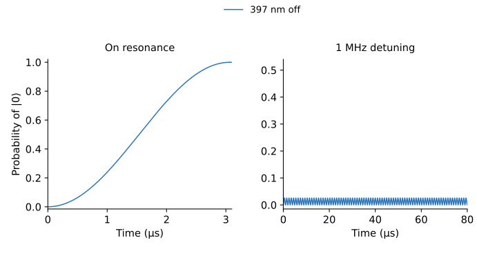

With 397 nm off, two panels show D-state population for resonant and 1 MHz detuned 729 nm driving. The resonant pulse transfers nearly all population in about 3.07 microseconds; the detuned population remains below 2.6 percent over 80 microseconds.

Now add the measurement beam (here I use $\Omega_{397}=\Gamma/2$ as a reference power):

with_measurement = [population(d, Gamma / 2, t)
                    for d, t in zip(detunings, times)]

The orange curves in the plot below show what happens when both beams are turned on simultaneously:

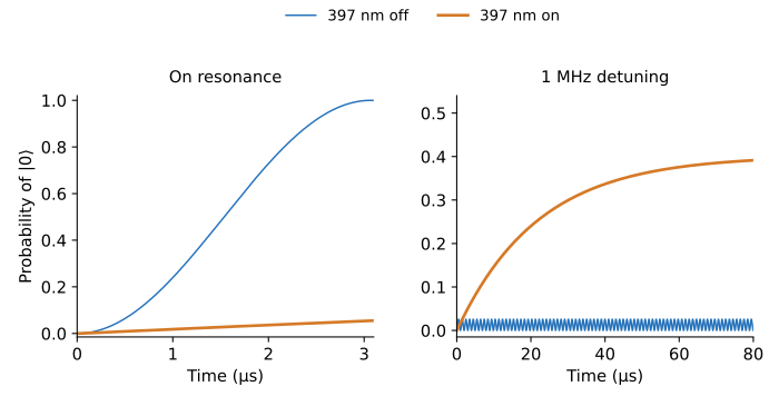
Matched full three-level simulations with 397 nm off in blue and on in orange. Measurement light suppresses the initial resonant Rabi flop to about 5.5 percent at the pi-pulse time and enhances the 1 MHz detuned population to about 39 percent after 80 microseconds.

On resonance, the measurement beam suppresses the initial transfer: at the usual π-pulse time, only about 5% of the population is in D. Off resonance, it does the opposite: the D population reaches about 40% after 80 µs, far above the coherent bound of 2.6%.

The physics

What causes this physically? The simplest toy model is a continuously driven two-level system, where Rabi oscillations are interleaved with repeated ideal S/D measurements, averaging over both outcomes:

Delta = 2 * np.pi * 1e6     # set this to zero to model on resonance
dt = 0.1e-6                # ideal state measurement every 0.1 microseconds
frequency = np.sqrt(Omega**2 + Delta**2)
p_step = (Omega / frequency)**2 * np.sin(frequency * dt / 2)**2

p_D = 0.0                  # start in S
probabilities = [p_D]
for _ in range(800):
    p_D = (1 - p_D) * p_step + p_D * (1 - p_step)
    probabilities.append(p_D)

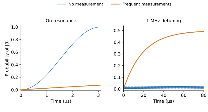
Two-state ensemble populations without measurement and with ideal S/D measurements every 0.1 microseconds. Measurements suppress resonant transfer to about 7.4 percent at the pi-pulse time and enhance the 1 MHz detuned population to about 49 percent after 80 microseconds.

On resonance, this is the familiar quantum Zeno effect. In each short interval, the ion develops only a small probability of being in D. A measurement therefore usually finds it still in S, putting it back at the starting point. Repeating these checks interrupts the coherent buildup needed to complete a Rabi flop.

Off resonance, the effect is less familiar. Without measurement, the excitation amplitudes coherently cancel over time, resulting in low population transfer. The measurements interrupt the cancellation and allow population to build up. This is anti-Zeno enhancement. It is not unlimited: sufficiently rapid measurements eventually suppress transfer here too.

One way to test this interpretation is to replace the repeated measurements with repeated random phase updates. Here is what it looks like on the Bloch sphere at 1 MHz detuning. A perfectly coherent laser phase keeps the state on a small orbit near S. Random phase updates change the rotation axis, allowing the state to move much further from S.

The two toy models agree on the average populations, but the single phase history on the right is not a photon-conditioned quantum trajectory.

Animated Bloch spheres at 1 MHz detuning: a fixed laser phase keeps the state near S, while random phase updates every 0.1 microseconds let it move farther away. The right sphere follows one pure-state phase history; the orange population curve is the ensemble average, not a fluorescence record.

This is a fancy way of saying something familiar: for a quantum gate, we want a narrow linewidth and a stable phase throughout the pulse. However, if we only want off-resonant population transfer, a broader, always-on drive can help, with coherent Rabi oscillations giving way to rate equations. The twist in our setting is that the measurement itself broadens the transition, even if the laser linewidth is very low.

Answering the original puzzle

Special thanks to Tyler Sutherland for helping me piece this together, and congratulations to David Nadlinger, who solved the puzzle in the comment section of last week’s post.

In the previous post, I asked: how far do I have to detune the 729 nm beam to keep the D-state excitation probability below $10^{-5}$? For a perfectly coherent drive, the maximum population is

\[p_{D,\max}=\frac{\Omega^2}{\Omega^2+\Delta^2}.\]

With $\Omega/(2\pi)\approx163$ kHz, that gave an answer of about 51.5 MHz, regardless of pulse duration. So why was this not what I observed experimentally?

The answer: the always-on qubit laser is also necessarily on during dissipative operations, such as measurement or cooling. The scattering during those operations enhances the probability of a D-state excitation through the anti-Zeno effect.

Let’s ballpark this quantitatively. In the limit of weak, fast fluorescence, we can eliminate the short-lived P state and describe its effect as loss of S–D coherence. If the bright ion emits at rate $R$, this gives

\[\gamma_\phi=\frac{R}{2}, \qquad B=\frac{\gamma_\phi}{\pi}=\frac{R}{2\pi}.\]

Here $\gamma_\phi$ is the coherence-decay rate, and $B$ is the equivalent Lorentzian full width at half maximum in Hz. The rate $R$ counts all emitted photons while the ion is bright, including the ones we do not detect. For ⁴⁰Ca⁺ at the 397 nm reference power above, $\Omega_{397}=\Gamma/2$, we find an effective linewidth of 3.8 MHz due to measurement, over one million times larger than the natural linewidth of the qubit transition! At this power, the linewidth analogy gives the far-detuned excitation rate; it is not an exact description of the full three-level system near resonance.

Using the standard rate-equation approximation (Eq. 8), assuming $\gamma_\phi\gg\Omega$ and neglecting D-state decay, the stimulated transition rate in this effective two-level model is

\[W(\Delta)=\frac{\Omega^2\gamma_\phi}{2(\Delta^2+\gamma_\phi^2)}.\]

Starting in S, far from resonance ($\lvert\Delta\rvert\gg\gamma_\phi,\Omega$), the population after the initial coherence transient and before appreciable transfer ($Wt\ll1$) or D-state decay ($t\ll\tau_D$) is approximately

\[p_D(t)\simeq Wt \simeq\frac{Rt}{4}\left(\frac{\Omega}{\Delta}\right)^2.\]

The important change is the factor of time. The coherent excitation stays bounded; during scattering, small amounts of unwanted population can keep accumulating. For example, at $t=1\,\mathrm{ms}$, we find:

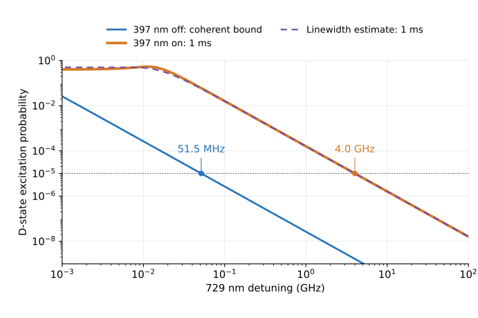
D-state excitation versus 729 nm detuning. The coherent bound with 397 nm off is blue; the full three-level population after 1 ms with 397 nm on is orange; the linewidth estimate is dashed purple. Reaching the same target of 10 to the minus 5 requires about 51.5 MHz for the coherent bound and 4.0 GHz with measurement light.

We’re now in a position to answer the puzzle. Previously, we thought that detuning the 729 nm laser by 51.5 MHz would keep the D-state excitation probability below $10^{-5}$, but it doesn’t when the measurement beam is also on. Instead, we have to account for the total duration of the relevant measurement and cooling steps, using the formula above. For a 1 ms measurement at the reference power in this model, we require about 4.0 GHz detuning, roughly 80 times the first answer.

That was the missing piece. Keeping the power constant solved the charging problem, but the light that measured and cooled the ion also removed the protection I thought detuning would provide. No free lunch, I guess!