Down with T2, long live T3!
One of the main metrics used to describe a quantum computer is qubit coherence time, typically denoted as $T_2$. There is just one problem: $T_2$ is pretty useless at predicting the effect of qubit decoherence on computational errors! In this post, I explain why that is, and argue for adopting a new coherence measure more fit for the task: $T_{3}$.
Primer on qubit coherence
Qubit coherence is typically measured using a Ramsey sequence, when a qubit is prepared in a superposition of 0 and 1 and subjected to free-evolution of duration $t$ before it’s measured in the computational basis. The corresponding quantum circuit looks as follows:
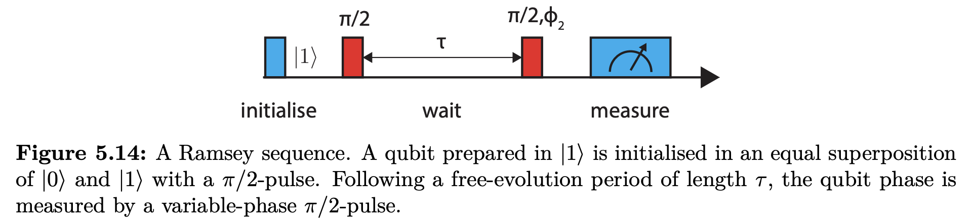
The coherence time - typically denoted as $T_2^*$ or $T_2$, depending on your community - is the maximum value of $t$ for which this superposition “remains quantum”. More precisely, it is the time $t$ for which the probability of obtaining the correct result drops by $0.5 \times (1 - 1/e) \approx 32\%$.
It is frequently possible to extend the coherence time by manipulating the qubit during the free-evolution time. Scientists will often report the coherence time - which they might call $T_2$ or $T_{2, echo}$, depending on the community - measured while attempting to stabilise the qubit state in this fashion, either using a single “spin echo” pulse, or using a more involved “dynamical decoupling” sequence. Either way, the intuition is that $T_2$ is the time over which the “quantumness” of a quantum state can be maintained.
What’s the issue?
So far, so good, but there is a caveat. In quantum computing, it is generally necessary for all the operations to be performed with fidelity above $\approx 99.9\%$. Consequently, the longest acceptable delay must introduce an error with probability $< \approx 0.1\%$. That is the number we need to figure out about our quantum computer. However, $T_2$ only tells us about the length of delay that introduces an error with probability $\approx 63\%$ - waaaaaay longer than any delay we actually want to introduce.
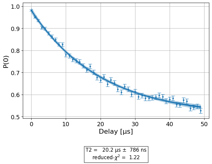
The way most scientists approach this challenge is that they measure $T_2$ and extrapolate down to the timescale of interest. You could, following the example in Qiskit’s tutorials, perform the Ramsey measurement, fit $P= A \exp(-t/T_2) + B$, and then calculate $P(t_0)$ to calculate the error associated with a delay time $t_0$. For such exponential decay, we’d expect to get $\approx 0.1\%$ error for a wait time $t \approx 0.001 \times T_2$.
However, this method is unfortunately pretty terrible at getting more than an order-of-magnitude estimate for an error in the range of 0.1%. There are several reasons for this:
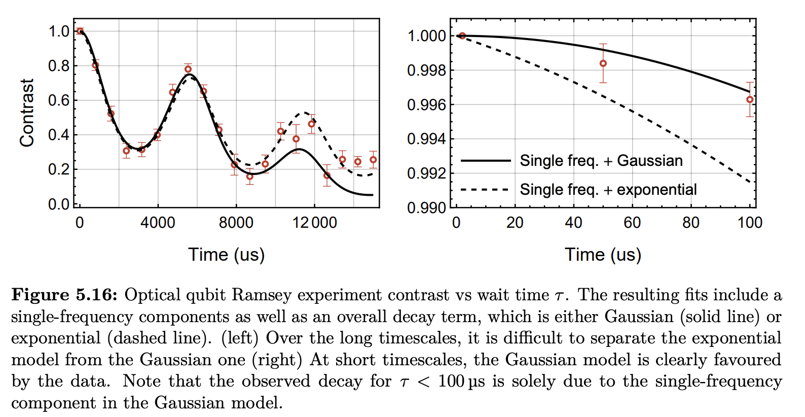
- Noise spectrum. Each fit function to the Ramsey sequence assumes a certain noise spectrum, e.g. white noise in the case of the exponential fit. However, that is always an approximation, and it is very common for the noise spectrum to vary dramatically between the short timescales (relevant for 0.1% level errors) and long timescales (relevant for 68% level errors).
- Fit uncertainty. Even eyeballing the graph above, it is clear that it would take a lot more data to measure $P(0)$ with an error much lower than 0.1% than it takes to establish $T_2$ to a reasonable accuracy.
To summarise the issue:
- In a quantum computer, all relevant delays and operations must occur at or below a timescale $t_0$ where the probability of decoherence $1-P(t_0)$ is less than approximately 0.1%
- To measure $P$ vs $t$ in the high-fidelity regime, it is fairly useless to measure $P$ vs $t$ in the low-fidelity regime, as is typical for $T_2$ measurement.
What’s the solution?
I believe the time has come to adopt a new coherence metric, more fit for the quantum computing era. I propose that in addition to $T_2$ (or even instead of $T_2$!), quantum computing papers start systematically measuring and reporting what I call $T_{3}$ - the maximum delay over which the superposition fidelity remains above three nines (hence the name).
So how do you actually measure $T_{3}$? It is possible to do it using a standard Ramsey sequence with a short delay time, though it takes time, and one has to be careful about subtracting state preparation and measurement (SPAM) errors. During my PhD work, I was able to take the following data, which put $T_{3}$ somewhere around 50 us:
A way better approach was pioneered by the group of John Martinis in 2015. Here, delay times are interleaved inside a single-qubit randomised benchmarking sequence. This serves to significantly amplify the delay errors, reducing the statistical uncertainty and hence the data acquisition time.
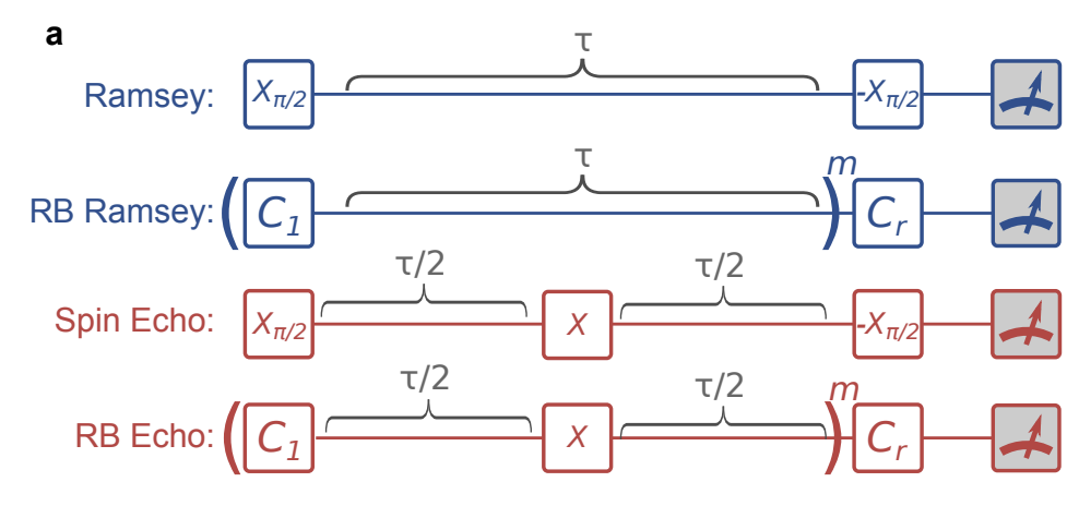
This technique allowed O’Malley et al to obtain the following result, indicating $T_{3} \approx 50$ ns.
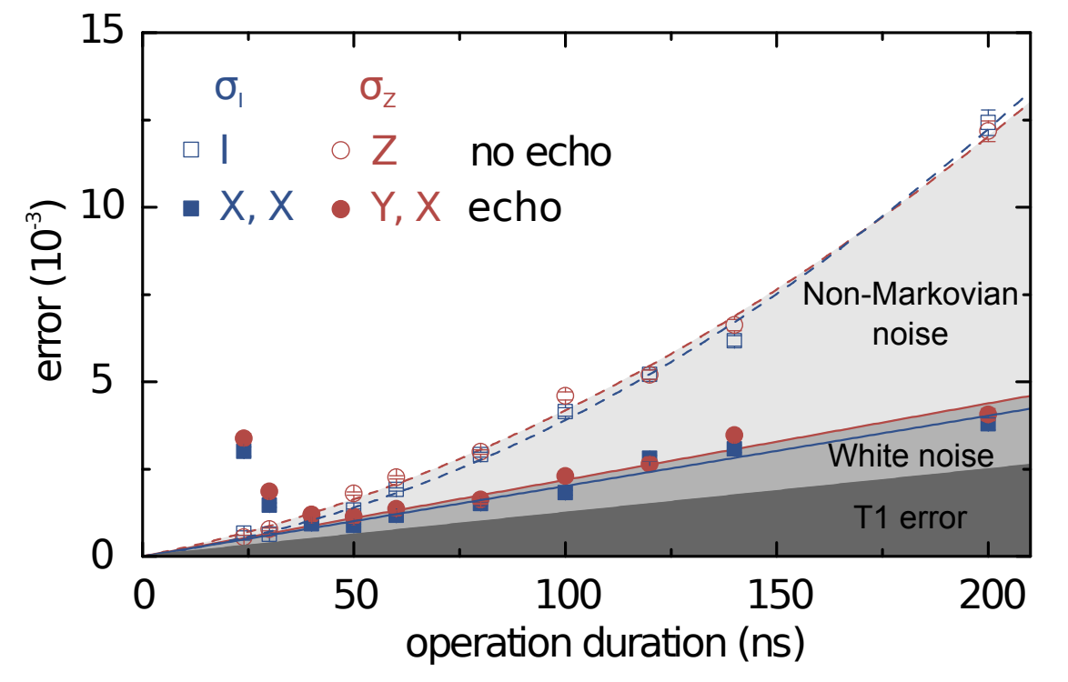
Another insight that immediately comes out of such results is that while dynamical decoupling may be a great way of extending $T_2$, it is not always a great way of extending $T_{3}$. For example, in the plot above, we see that spin echo suppresses noise at $t > 50$ ns, but introduces extra noise for $t < 40$ ns. This is not uncommon - is it really easy to unintentionally inject 0.1% of error, e.g. due to amplitude noise in the dynamical decoupling drive!
The approach from O’Malley et al was then adopted by David Lucas’s trapped ion group in Oxford, with the result presented in Sepiol et al 2019:
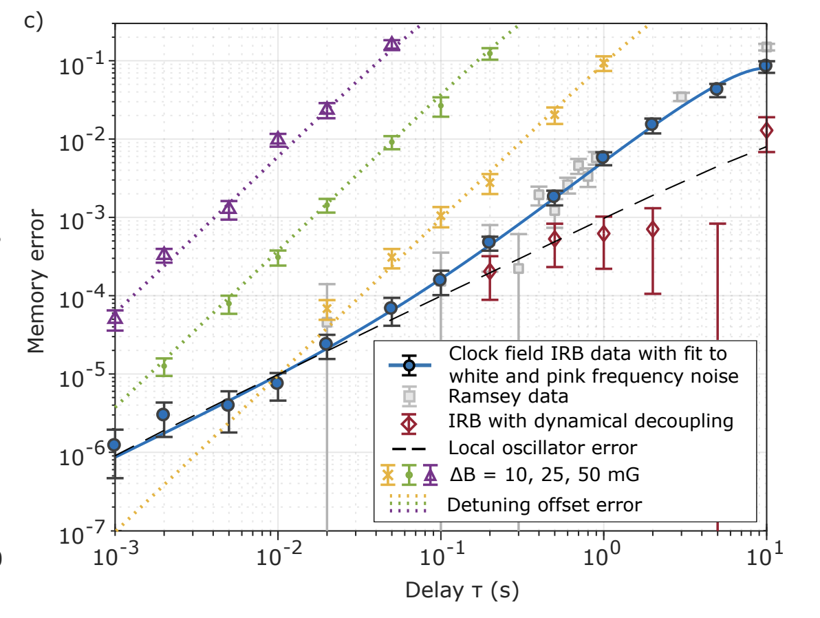
This graph may look overwhelming, but here is the gist. Sepiol et al use the error amplification technique to measure idling errors as low as $10^{-6}$. By sitting at the magnetic-field-insensitive point of their qubit, and without any spin echo (blue points), the authors record $T_{3} \approx 0.4$ s (that’s right: 400 ms). And by employing dynamical decoupling (red points), they can keep the memory error to < 0.1% for $T_{3} \approx 5$ s - although this number comes with an understandably large error bar.
The method has since been very popular in Oxford, including where I work at Oxford Ionics, where it allowed us to study qubit dephasing in preparation for our ultra-high fidelity two-qubit gates demo in 2024 (NB this was at the 99.99% level, so we’re even talking about $T_{4}$ now!). Quantinuum also adopts a variant of this method to measure errors during ion transport, to which qubit decoherence is a major contributor. For example, in the H2 paper they report “transport 1Q RB” error of $2 \times 10^{-3}$ for a delay duration of $\approx 60$ ms (I estimated this from Table I). So while they don’t report it exactly, I give them an honourable mention with $T_{3} \approx 30$ ms. Please correct me if I got that number wrong!
Despite these examples, O’Malley et al’s approach has not been widely adopted in the QC community since its proposal a decade ago. I think that’s a shame, and I hope this post helps spread the word about this technique.
So what do you think about $T_{3}$? Are you going to measure it in your system (and cite this blog post appropriately)? Do let me know in the comments.