By now, we have all seen how AI software engineers, AI chatbots, and AI copywriters change the game. In this blog series, I wanted to go broader, and extrapolate from my personal and professional experiences in quantum computing on how AI will impact deep tech R&D. This post is part 1, which is all about how crazy good AI can be at doing everyday physics .
Ok, I say it’s a blog series, but knowing myself… who knows when, if ever, I’ll get round to writing a follow-up. But for now, enjoy this raw footage of AI agents:
- Totally nailing maths questions that stumped me during my PhD
- Doing monte-carlo simulations of blackbody radiation on cryogenic cows
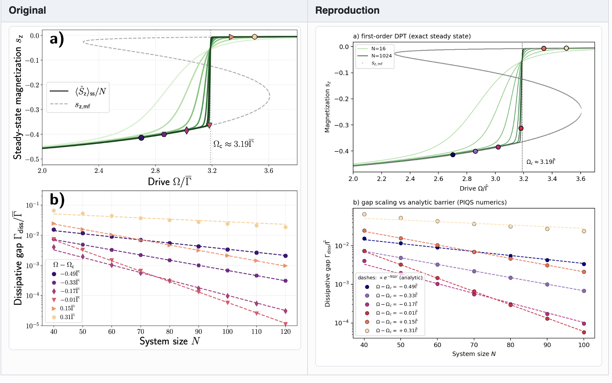
- Reproducing the results on my messy paper from 2017
- Nailing the quantum computing state-of-the-art literature research
Section A: AC Stark shifts
Question. Hey AI, I have a following problem for you. It is well known that if I resonantly drive a transition within a multi-level system, the frequency of that transition is shifted by the AC Stark/Zeeman shift of spectator levels. I know very well how to prove that a 2-level system driven off resonance experiences a frequency shift of $\approx \Omega^2/(4\delta)$. However, evenever I had tried to derive this for a 3-level system - where one of the transitions is driven on resonance, and one of the transitions is driven off resonance - I had failed. Can you help me out?
Mathematically, the problem boils down to finding the eigenvalues of the Hamiltonian
\[H/\hbar = \begin{pmatrix}
0 & \Omega_1/2 & \Omega_2/2 \\
\Omega_1/2 & -\delta & 0 \\
\Omega_2/2 & 0 & \Delta-\delta
\end{pmatrix},\]
in the basis $(\lvert 0\rangle, \lvert 1\rangle, \lvert e\rangle)$. This represents a qubit drive $\lvert 0\rangle \leftrightarrow \lvert 1\rangle$, with Rabi frequency $\Omega_1$ which also couples $\lvert 0\rangle \leftrightarrow \lvert e\rangle$, but that transition is detuned by $\Delta$ and has Rabi frequency $\Omega_2$. Again, I expect to see that the eigenvalue corresponding to the $\lvert 0\rangle \leftrightarrow \lvert 1\rangle$ dressed state experiences a shift of $\approx \Omega_2^2/(4\delta)$ compared to a two-level system.
AI answer. The goal is to confirm that turning on a far-detuned drive $\lvert 0\rangle \to \lvert e\rangle$ with Rabi frequency $\Omega_2$ shifts the qubit ($\lvert 0\rangle \leftrightarrow \lvert 1\rangle$) dressed-state energies by an amount of order $\Omega_2^2/(4\Delta)$, where $\Delta$ is the large detuning of the second drive. Derive the result carefully (the user reports their analytics didn’t close) and then verify numerically by diagonalizing the full $3\times 3$ Hamiltonian.
1. Hamiltonian and conventions
In the basis ${\lvert 0\rangle, \lvert 1\rangle, \lvert e\rangle}$ and with $\hbar = 1$,
\[H = \begin{pmatrix}
0 & \Omega_1/2 & \Omega_2/2 \\
\Omega_1/2 & -\delta & 0 \\
\Omega_2/2 & 0 & \Delta - \delta
\end{pmatrix}.\]
This is the standard rotating-frame Hamiltonian for two simultaneous drives sharing the ground state $\lvert 0\rangle$. The $\lvert 0\rangle \leftrightarrow \lvert 1\rangle$ drive (qubit) is nearly resonant, with small detuning $\delta$ and Rabi frequency $\Omega_1$. The $\lvert 0\rangle \leftrightarrow \lvert e\rangle$ drive is far off-resonant, with large detuning $\Delta$ and Rabi frequency $\Omega_2$.
A useful sign-convention check: with no couplings ($\Omega_1=\Omega_2=0$) the diagonal energies in this frame are $E_{\lvert 0\rangle}=0$, $E_{\lvert 1\rangle}=-\delta$, $E_{\lvert e\rangle}=\Delta-\delta$. A positive $\Delta$ means $\lvert e\rangle$ sits well above $\lvert 0\rangle$ in the rotating frame, so the $\lvert 0\rangle$-light shift from $\lvert e\rangle$ should be negative (level repulsion from above).
Throughout we take $\Delta \gg \Omega_1, \Omega_2, \lvert\delta\rvert$ and assume $\Delta - \delta \approx \Delta$ wherever convenient (we keep $\Delta - \delta$ where it matters).
2. Bare 2-level dressed states ($\Omega_2 = 0$)
With $\Omega_2 = 0$, the third level decouples and the ${\lvert 0\rangle, \lvert 1\rangle}$ block
\[H_2^{(0)} = \begin{pmatrix} 0 & \Omega_1/2 \\ \Omega_1/2 & -\delta \end{pmatrix}\]
has the textbook dressed-state eigenvalues
\[E_\pm^{(0)} = -\frac{\delta}{2} \pm \frac{1}{2}\sqrt{\delta^2 + \Omega_1^2}\]
(generalized Rabi frequency $\Omega_R = \sqrt{\delta^2+\Omega_1^2}$). On resonance ($\delta=0$) these become $E_\pm^{(0)} = \pm \Omega_1/2$.
3. Adiabatic elimination of $\lvert e\rangle$
There are two equivalent ways to derive the effective Hamiltonian for the qubit manifold; both expose the sign and position of the shift cleanly.
3.1 Second-order Rayleigh–Schrödinger perturbation theory
Split $H = H_0 + V$ with
\[H_0 = \mathrm{diag}(0, -\delta, \Delta-\delta), \qquad V = \begin{pmatrix} 0 & \Omega_1/2 & \Omega_2/2 \\ \Omega_1/2 & 0 & 0 \\ \Omega_2/2 & 0 & 0 \end{pmatrix}.\]
Standard second-order perturbation for level $\lvert n\rangle$ gives $\Delta E_n^{(2)} = \sum_{m\ne n} \lvert V_{nm}\rvert^2/(E_n^{(0)} - E_m^{(0)})$.
We do not treat $\Omega_1$ as perturbative — we keep the $\Omega_1/2$ coupling exactly. The perturbative parameter is the small ratio $\Omega_2/\Delta$, so we only eliminate matrix elements that couple to $\lvert e\rangle$. Within the ${\lvert 0\rangle, \lvert 1\rangle}$ subspace, the effect of $\lvert e\rangle$ at leading (second) order is to renormalize the diagonal entries. On $\lvert 0\rangle$ (energy $0$), $\Delta E_{\lvert 0\rangle} = \lvert\Omega_2/2\rvert^2/(0 - (\Delta-\delta)) = -\Omega_2^2/(4(\Delta-\delta))$. On $\lvert 1\rangle$ (energy $-\delta$), there is no direct coupling to $\lvert e\rangle$ in $V$, so $\Delta E_{\lvert 1\rangle} = 0$ at this order.
The cross term $V_{0e}V_{e1}$ vanishes because $V_{e1}=0$. So no off-diagonal correction appears at second order in $\Omega_2$.
The punchline: the light shift sits entirely on $\lvert 0\rangle$, with magnitude
\[s \equiv \frac{\Omega_2^2}{4(\Delta-\delta)} \approx \frac{\Omega_2^2}{4\Delta},\]
and sign such that $\lvert 0\rangle$ moves toward lower energy when $\Delta > 0$ (i.e., when $\lvert e\rangle$ is above $\lvert 0\rangle$).
3.2 Same result by explicit projection / Schrieffer–Wolff
Write $\lvert\psi\rangle = c_0\lvert 0\rangle + c_1\lvert 1\rangle + c_e\lvert e\rangle$, project $H\lvert\psi\rangle = E\lvert\psi\rangle$ onto $\lvert e\rangle$, and solve adiabatically for $c_e$ assuming $\lvert\Delta - \delta - E\rvert \approx \Delta$:
\[(\Delta - \delta) c_e + \frac{\Omega_2}{2} c_0 = E c_e \;\Longrightarrow\; c_e \approx -\frac{\Omega_2/2}{\Delta - \delta} c_0.\]
Substituting back into the $\lvert 0\rangle$ row gives an effective $\lvert 0\rangle$-energy correction of $-\Omega_2^2/[4(\Delta-\delta)]$, in agreement with section 3.1.
3.3 Effective 2-level Hamiltonian
The qubit subspace is therefore governed by
\[H_\mathrm{eff} = \begin{pmatrix} -s & \Omega_1/2 \\ \Omega_1/2 & -\delta \end{pmatrix}, \qquad s = \frac{\Omega_2^2}{4(\Delta-\delta)}.\]
The Rabi coupling $\Omega_1$ is unmodified at this order (there is no $\lvert 1\rangle \leftrightarrow \lvert e\rangle$ matrix element to generate one).
4. Modified dressed-state energies
Diagonalising $H_\mathrm{eff}$:
\[E_\pm = -\frac{\delta + s}{2} \pm \frac{1}{2}\sqrt{(\delta - s)^2 + \Omega_1^2}.\]
Compare with the bare result $E_\pm^{(0)} = -\delta/2 \pm \frac{1}{2}\sqrt{\delta^2+\Omega_1^2}$. Two distinct effects appear. First, a common shift $-s/2$ on the mean of the dressed-state pair. This is the “$\Omega_2^2/(4\Delta)$ shift” the user is asking about, but divided by 2 because the $\lvert 0\rangle$-character is split between the two dressed states. Second, a modified generalised Rabi frequency $\Omega_R \to \sqrt{(\delta-s)^2 + \Omega_1^2}$, i.e. the effective qubit detuning becomes $\delta_\mathrm{eff} = \delta - s$.
4.1 On resonance ($\delta = 0$)
Expanding in $s/\Omega_1$:
\[E_\pm = -\frac{s}{2} \pm \frac{1}{2}\sqrt{s^2 + \Omega_1^2} \approx -\frac{s}{2} \pm \frac{\Omega_1}{2}\left(1 + \frac{s^2}{2\Omega_1^2}\right).\]
So both dressed states shift by $-s/2 = -\Omega_2^2/[8(\Delta-\delta)]$, and the splitting between them changes only at the much smaller order $s^2/\Omega_1$ (i.e., $\Omega_2^4/(\Delta^2 \Omega_1)$). The qubit transition frequency $E_+ - E_-$ is essentially immune to the light shift on resonance; what shifts is the absolute position of the doublet.
4.2 Answer to the user’s question (signs and where it lives)
The $\Omega_2^2/(4\Delta)$ shift lives on $\lvert 0\rangle$ in the bare basis. In the dressed basis it does not appear symmetrically with the full magnitude on both states. On resonance it splits 50/50, giving a common shift of $-\Omega_2^2/[8\Delta]$ to each dressed state. Off resonance, the state with more $\lvert 0\rangle$ character takes a larger share. The sign is negative when $\Delta > 0$ (the second level is above $\lvert 0\rangle$ in the rotating frame, so it pushes $\lvert 0\rangle$ down).
So the user’s intuition was right in magnitude and parametric scaling but slightly off in distribution: each dressed state moves by only half the bare-$\lvert 0\rangle$ light shift.
5. Numerical verification
A script diagonalises the full $3\times 3$ Hamiltonian and compares against (a) the bare 2-level prediction (ignores $\Omega_2$) and (b) the effective 2-level Hamiltonian after adiabatic elimination.
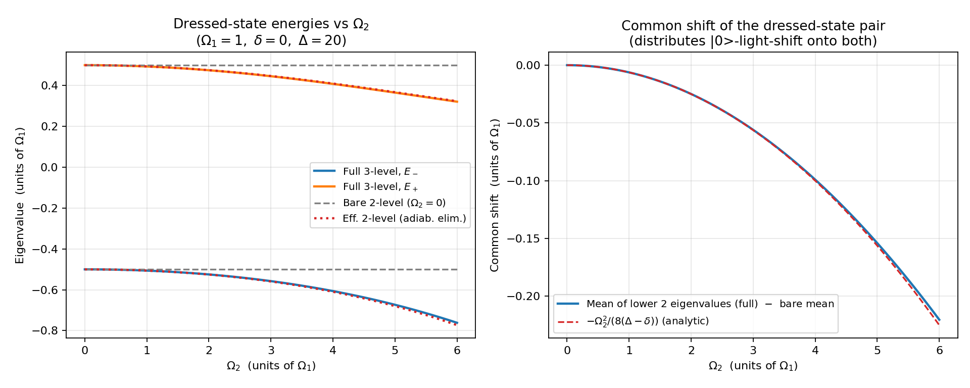
5.1 Dressed energies vs $\Omega_2$
For parameters $\Omega_1 = 1$, $\delta = 0$, $\Delta = 20\,\Omega_1$, the two qubit-like eigenvalues of the full 3-level Hamiltonian bend downward as $\Omega_2$ grows. The bare 2-level prediction (flat at $\pm 0.5$) ignores the light shift entirely and quickly fails. The adiabatic-elimination prediction sits essentially on top of the full result over the whole sweep. The mean of the lower two eigenvalues, minus the bare mean, matches the analytic prediction $-s/2 = -\Omega_2^2/[8(\Delta-\delta)]$ to plotting precision.
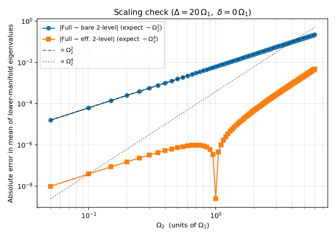
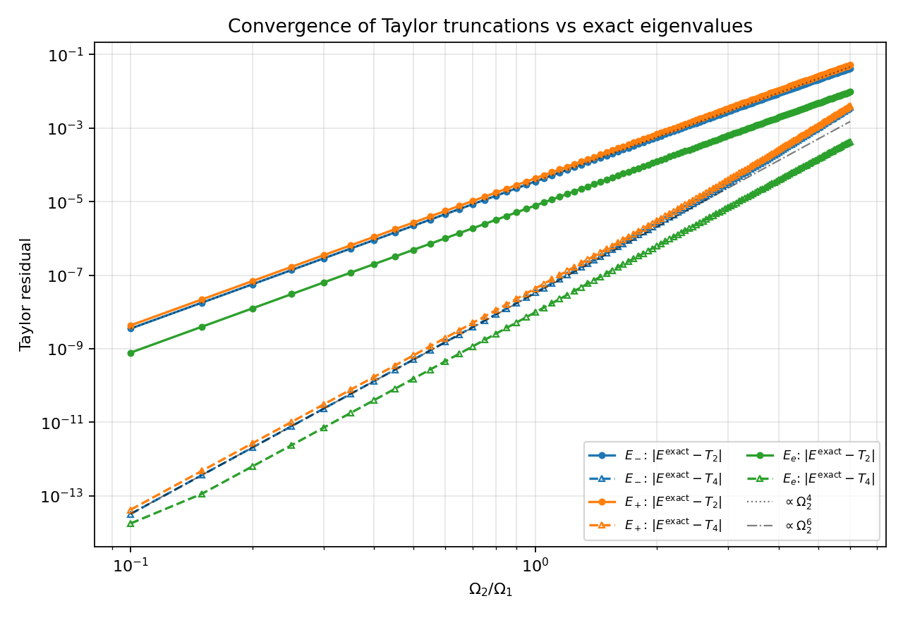
5.2 Scaling check
The log-log error plot is the cleanest way to confirm the perturbative structure. The error of the bare 2-level approximation lies exactly on the reference $\propto \Omega_2^2$ slope — this is the AC Stark shift. The error of the effective 2-level approximation tracks the $\propto \Omega_2^4$ reference. The effective Hamiltonian captures the $\Omega_2^2/\Delta$ correction at leading order in $1/\Delta$ — the exact second-order shifts (derived in Section 6) carry energy denominators $\lambda_0 - (\Delta-\delta)$ rather than $\Delta-\delta$, so there is a smaller residual already at order $\Omega_2^2$ from the neglected $\lambda_0/\Delta$ dependence. For the plotted parameters ($\Delta = 20\,\Omega_1$) that subleading piece is numerically tiny and partly cancels in the mean of the lower manifold, so the observed slope remains $\Omega_2^4$. Section 6 gives the cleaner / more rigorous statement.
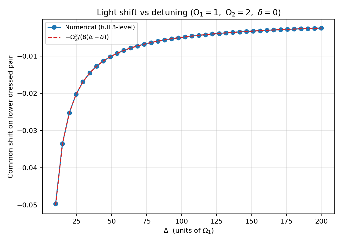
5.3 Scaling with $\Delta$ at fixed $\Omega_2$
For $\Omega_1=1$, $\Omega_2 = 2$, $\delta = 0$, $\Delta \in [10, 200]$, the common shift of the dressed pair tracks $-\Omega_2^2/[8(\Delta-\delta)]$ across nearly two orders of magnitude in $\Delta$, with no free parameters. This is the $1/\Delta$ signature of an off-resonant light shift.
5.4 Numerical table
For the resonant case $\delta=0$, $\Omega_1=1$, $\Delta=20$:
| $\Omega_2$ |
$E_-$ (full) |
$E_+$ (full) |
$E_e$ (full) |
predicted per-state shift $-s/2$ |
| 0 |
-0.5000 |
0.5000 |
20.000 |
0.0000 |
| 1 |
-0.5061 |
0.4936 |
20.0125 |
-0.00625 |
| 2 |
-0.5250 |
0.4750 |
20.0499 |
-0.02500 |
| 3 |
-0.5577 |
0.4458 |
20.1119 |
-0.05625 |
| 4 |
-0.6064 |
0.4082 |
20.1982 |
-0.10000 |
| 5 |
-0.6735 |
0.3656 |
20.3080 |
-0.15625 |
| 6 |
-0.7617 |
0.3211 |
20.4406 |
-0.22500 |
At $\Omega_2 = 2$: the bare doublet ${-0.5, +0.5}$ becomes ${-0.525, +0.475}$, a common shift of $-0.025 = -\Omega_2^2/[8(\Delta-\delta)]$. The $\lvert e\rangle$-like state has moved up by $+\Omega_2^2/[4\Delta] = +0.05$ — the opposite shift, as required by trace conservation of $H$.
6. Exact eigenvalues and Taylor-expansion cross-check
Sections 3–4 derived the light shift by adiabatically eliminating $\lvert e\rangle$. That’s clean but perturbative in $\Omega_2/\Delta$. Here we check the result the other way round: write down the exact eigenvalues of the full $3\times 3$ Hamiltonian (as roots of a cubic), then Taylor-expand in $\Omega_2$ and confirm the leading correction reproduces — and the next-order term predicts — the adiabatic-elimination answer.
A sympy script does all of this symbolically.
6.1 Characteristic polynomial
\[P(\lambda) = \det(\lambda I - H) = \lambda^3 + \lambda^2(2\delta - \Delta) + \lambda\left[\delta^2 - \delta\Delta - \frac{\Omega_1^2 + \Omega_2^2}{4}\right] + \frac{\Omega_1^2(\Delta-\delta)}{4} - \frac{\Omega_2^2 \delta}{4}.\]
Trace check: $-\mathrm{coeff}(\lambda^2) = \Delta - 2\delta = \mathrm{Tr}\,H$. Determinant check: $P(0) = -\det H$, so $\det H = -\Omega_1^2(\Delta-\delta)/4 + \Omega_2^2\delta/4$. Direct expansion of $H$ along the first row gives the same value (sanity check: at $\Omega_1 = 2, \Omega_2 = 0, \delta = 0, \Delta = 4$, $\det H = -4$, and $-\Omega_1^2(\Delta-\delta)/4 = -4$).
6.2 Factorisation at $\Omega_2 = 0$
\[P_0(\lambda) \equiv P(\lambda)\big\rvert_{\Omega_2=0} = (\lambda - (\Delta-\delta))(\lambda^2 + \delta\lambda - \Omega_1^2/4).\]
The quadratic factor is the bare 2-level block. So at $\Omega_2 = 0$ the three eigenvalues are the bare dressed states $E_\pm^{(0)} = -\delta/2 \pm \frac{1}{2}\sqrt{\delta^2 + \Omega_1^2}$ and the bare excited level $E_e^{(0)} = \Delta - \delta$. The full polynomial differs from $P_0$ by
\[P(\lambda) - P_0(\lambda) = -\frac{\Omega_2^2}{4}(\lambda + \delta),\]
which is the only way $\Omega_2$ enters. Note in particular that $P$ depends on $\Omega_2$ only through $\Omega_2^2$, so every eigenvalue is an even function of $\Omega_2$ — the Taylor series contains only $\Omega_2^{2n}$ terms.
6.3 Implicit-function theorem ⇒ perturbation series
Write $\lambda = \lambda_0 + \lambda_2 \Omega_2^2 + \lambda_4 \Omega_2^4 + \cdots$ with $\lambda_0$ one of the three bare roots, expand $P(\lambda, \Omega_2) = 0$, and match powers of $\Omega_2$. The first two orders give
\[\lambda_2 = \frac{\lambda_0 + \delta}{4 P_0'(\lambda_0)}, \qquad \lambda_4 = \frac{\lambda_2/4 - \frac{1}{2} P_0''(\lambda_0) \lambda_2^2}{P_0'(\lambda_0)}.\]
For a monic cubic, $P_0’’’$ is a constant, so these two terms close the system through $\mathcal{O}(\Omega_2^4)$.
Evaluating at each bare root:
| branch |
$\lambda_0$ |
$\lambda_2$ |
| $E_+$ |
$-\delta/2 + \Omega_R/2$ |
$(\delta + \Omega_R)/[8\Omega_R((\delta+\Omega_R)/2 - \Delta)]$ |
| $E_-$ |
$-\delta/2 - \Omega_R/2$ |
$(\delta - \Omega_R)/[8\Omega_R(\Delta - (\delta-\Omega_R)/2)]$ |
| $E_e$ |
$\Delta - \delta$ |
$\Delta/(4\Delta(\Delta-\delta) - \Omega_1^2)$ |
where $\Omega_R \equiv \sqrt{\delta^2 + \Omega_1^2}$.
In the large-$\Delta$ limit ($\Delta \gg \Omega_1, \lvert\delta\rvert$):
\[\lambda_2^{(\pm)} \to -\frac{1}{8\Delta}\left(1 \pm \frac{\delta}{\Omega_R}\right), \qquad \lambda_2^{(e)} \to \frac{1}{4\Delta}.\]
Multiplying by $\Omega_2^2$, the leading shifts are
\[\Delta E_\pm = -\frac{\Omega_2^2}{8\Delta}\left(1 \pm \frac{\delta}{\Omega_R}\right), \qquad \Delta E_e = +\frac{\Omega_2^2}{4\Delta}.\]
This is exactly the result of Section 4, with the bonus that the $E_e$ shift comes out of the same expansion — its $+\Omega_2^2/(4\Delta)$ is the “missing partner” that makes the trace work.
6.4 Trace conservation, exactly
The sum of all three $\lambda_2$’s must vanish (since $\mathrm{Tr}\,H$ doesn’t depend on $\Omega_2$). This is a non-trivial identity at the level of the closed-form expressions above; sympy confirms sum(lam_2) = 0 and sum(lam_4) = 0.
In other words, the $\lvert 0\rangle$-light shift $-\Omega_2^2/(4\Delta)$ is distributed among the three eigenstates by weight — half each to $E_\pm$ on resonance, and the opposing $+\Omega_2^2/(4\Delta)$ to $E_e$ — but the total trace is preserved at every order in $\Omega_2$.
This is a cleaner statement than the level-by-level Section 3 result: adiabatic elimination appears to put the shift on $\lvert 0\rangle$ only, but that is a bare-basis statement; in the dressed basis the same shift gets sliced up according to the dressed-state composition, while $E_e$ moves the opposite way to balance the books.
6.5 Equivalence with the $\lvert c_0\rvert^2$ picture
The Section 6.3 expression for $\lambda_2$ can be rewritten in a more physically transparent form. The bare dressed state $\lvert\lambda_0\rangle$ has $\lvert 0\rangle$-amplitude $c_0$, where (for the $\pm$ states) $\lvert c_0^{(\pm)}\rvert^2 = \frac{1}{2}(1 \pm \delta/\Omega_R)$.
Standard second-order perturbation theory gives the shift from coupling $\langle 0\rvert V \lvert e\rangle = \Omega_2/2$:
\[\Delta\lambda_0 = \frac{\lvert c_0\rvert^2 (\Omega_2/2)^2}{\lambda_0 - E_e^{(0)}} = \frac{\lvert c_0\rvert^2 \Omega_2^2/4}{\lambda_0 - (\Delta - \delta)}.\]
In the large-$\Delta$ limit this is $-\lvert c_0\rvert^2 \cdot \Omega_2^2 / (4\Delta)$, i.e.
\[\Delta E_\pm = -\lvert c_0^{(\pm)}\rvert^2 \cdot \frac{\Omega_2^2}{4\Delta},\]
which is the same as the result above. The factor of $1/2$ that appears on resonance is just “$\lvert 0\rangle$ is half of each dressed state”.
6.6 Numerical verification
For $\Omega_1 = 1$, $\delta = 0$, $\Delta = 20\,\Omega_1$: the exact eigenvalue (from numerical diagonalization of the $3\times 3$) agrees with the Taylor series truncated at $\mathcal{O}(\Omega_2^2)$ — i.e. exactly the adiabatic-elimination prediction — out to $\Omega_2 \sim \Omega_1$. Including the next-order correction computed in Section 6.3 extends agreement to $\Omega_2 = 6\,\Omega_1$ (where $\Omega_2/\Delta = 0.3$, well outside the perturbative regime).
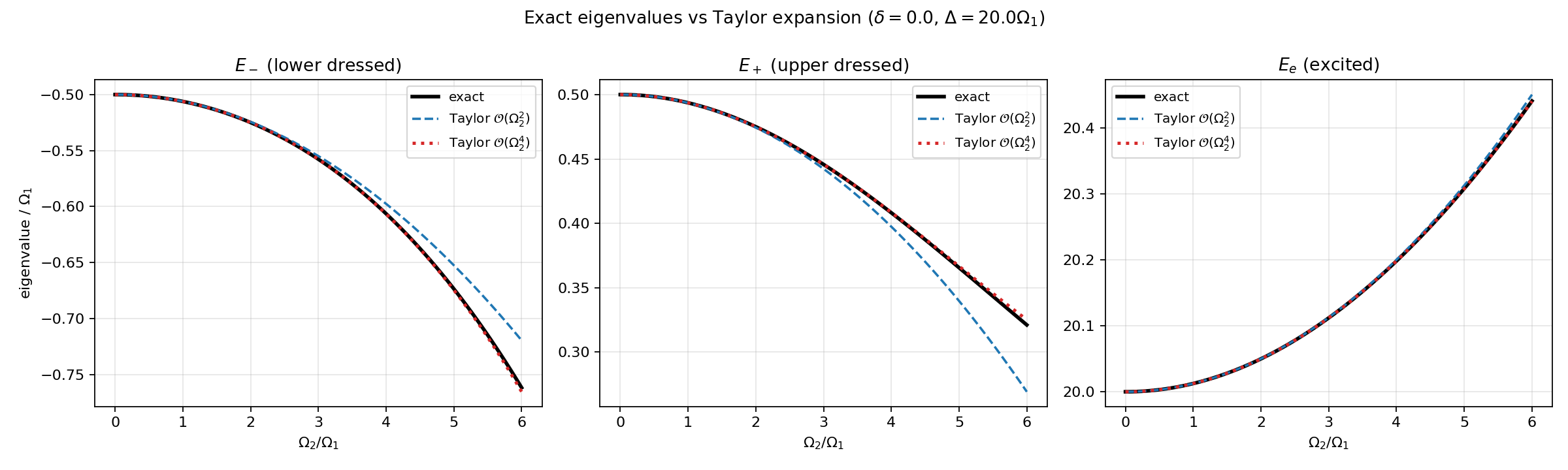
Log-log convergence: both the 2nd-order and 4th-order truncations behave as one expects from a Taylor series that only contains even powers of $\Omega_2$. The 2nd-order residual scales as $\Omega_2^4$ (the dropped next term); the 4th-order residual scales as $\Omega_2^6$ (the term after that). Reference $\Omega_2^4$ and $\Omega_2^6$ slopes confirm both scalings cleanly over three decades in $\Omega_2$. This is the strongest possible “the perturbative calculation was right” cross-check: not only does the leading shift match the adiabatic-elimination result, but the residual scales exactly as the next dropped Taylor term must.
6.7 What this adds over Section 5
Section 5 already showed numerically that the bare 2-level error scales as $\Omega_2^2$ and the adiabatic-elimination residual as $\Omega_2^4$. Section 6 shows analytically that the adiabatic-elimination Hamiltonian is the $\mathcal{O}(\Omega_2^2)$ truncation of the exact eigenvalue, and gives a closed-form expression for the next term. That term is the leading correction to the effective Hamiltonian if one wants to do better than adiabatic elimination — useful, e.g., for evaluating Stark-shift cancellation strategies at the $\Omega_2^4/\Delta^3$ level.
7. Summary
-
Derivation. Adiabatic elimination of $\lvert e\rangle$ gives an effective 2-level Hamiltonian for the qubit manifold in which $\lvert 0\rangle$ receives a light shift $-\Omega_2^2/[4(\Delta-\delta)]$ and $\lvert 1\rangle$ is unchanged (at this order). The off-diagonal qubit coupling $\Omega_1$ is also unchanged at this order.
-
Dressed eigenvalues. $E_\pm = -(\delta+s)/2 \pm \frac{1}{2}\sqrt{(\delta-s)^2 + \Omega_1^2}$ with $s = \Omega_2^2/[4(\Delta-\delta)]$. On resonance ($\delta=0$) each dressed state acquires a common shift of $-s/2 = -\Omega_2^2/[8\Delta]$; the dressed-state splitting is essentially unchanged (correction $\sim \Omega_2^4/(\Delta^2 \Omega_1)$).
-
User’s expected scaling. The $\Omega_2^2/(4\Delta)$ scaling is confirmed, with two refinements: (i) the shift sits on $\lvert 0\rangle$, not symmetrically on both dressed states; (ii) in the dressed basis each state receives only half the bare-$\lvert 0\rangle$ shift on resonance, because $\lvert 0\rangle$ is split 50/50 between $\lvert\pm\rangle$.
-
Numerics. Full $3\times 3$ diagonalization confirms the $-\Omega_2^2/[4(\Delta-\delta)]$ shift on $\lvert 0\rangle$ to the expected $O(\Omega_2^4/\Delta^2)$ relative accuracy, and the $1/\Delta$ scaling holds over the full range tested.
Section B: Black-body radiation
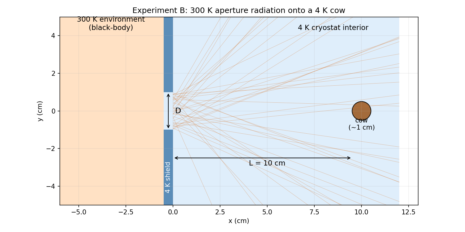
Question. Hey AI, I have a following problem for you. I have a little cow-shaped object, 1 cm in size. I want to put this cow in my 4K crystat, but I am worried about the cow heating up too much due to black body radiation through an aperture in the 4K heat shield 10 cm away, which looks directly at 300K. Draw this setup and calculate the total black body radiation on the cow as a function of aperture diameter. First, do this for a spherical object and compare numerical simulations with analytics. Then, repeat for a cow-shaped object. Assume the cow is centered with the aperture, and that the aperture looks at the cow from the side.
AI answer.
Setup
A 4 K shield with a circular aperture of diameter $D$ at $x=0$. A 1‑cm object (sphere or cow) sits at $x = L = 10$ cm. The cold side of the aperture acts as a Lambertian 300 K black body (Kirchhoff’s law: aperture into 300 K is indistinguishable from a 300 K black surface in the aperture plane). All emissivities are taken as $\varepsilon = 1$. 4 K self‑emission gives $\sigma T^4 = 1.45\times 10^{-5}$ W/m² vs $459$ W/m² at 300 K, a $3\times 10^{-8}$ ratio, so it is ignored.
1. Analytic sphere
Treating the sphere ($r=0.5$ cm) as a small target seen from a point on the aperture at off‑axis radius $\rho$, the hit‑probability density per unit aperture area is
\[f(\rho) = \frac{L r^2}{(L^2 + \rho^2)^{3/2}}\]
(Lambertian $\cos\theta$ projection times the solid angle of the sphere as seen from that aperture point). Integrating $2\pi\rho\,d\rho$ from $0$ to $D/2$:
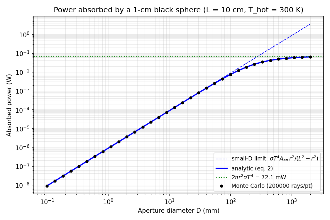
\[P(D) = 2\pi r^2 \sigma T^4 \left(1 - \frac{L}{\sqrt{L^2 + (D/2)^2}}\right).\]
Limiting behaviour: for a small aperture ($D \ll L$), $P \approx \sigma T^4 \cdot \pi(D/2)^2 \cdot r^2/L^2$ — pure aperture‑area scaling with the on-axis Lambertian view-factor $r^2/L^2$ (i.e. the point-target solid angle $\pi r^2/L^2$ divided by $\pi$, since the integrand $f(\rho)$ at $\rho=0$ is exactly $r^2/L^2$). For $r=0.5$ cm, $L=10$ cm this is $r^2/L^2 = 2.5\times 10^{-3}$. For a large aperture ($D \to \infty$), $P \to 2\pi r^2 \sigma T^4 \approx 72$ mW.
Note the factor of 2 in the asymptote. A naive “sphere in front of a black plane” estimate gives $\pi r^2 \sigma T^4$. The correct answer is $2\pi r^2 \sigma T^4$, because at infinite aperture the back hemisphere of the sphere also intercepts rays arriving from the (now arbitrarily large) aperture at glancing angles. I verified this independently with a separate surface‑integral Monte Carlo over a sphere in front of an infinite Lambertian half‑plane.
2. Sphere Monte Carlo
A naive uniform‑disc Lambertian Monte Carlo fails at large $D$ because the hit fraction falls to $\sim 10^{-5}$ and shot noise dominates. The code uses a cone‑importance sampler: stratify the aperture into log‑spaced annular rings; from each ring sample directions only within the cone that subtends the target’s bounding sphere; weight each ray by $(\cos\theta/\pi) \cdot \Omega_\mathrm{cone}$ — the Lambertian PDF divided by the uniform‑on‑cone PDF.
The Monte Carlo agrees with the analytic formula to $< 0.1\%$ across 8 decades in $D$.
3. Cow
A primitive cow mesh in trimesh: body ellipsoid + head sphere + four cylindrical legs + tail cylinder, bounding box diagonal 1 cm, broadside facing the aperture.
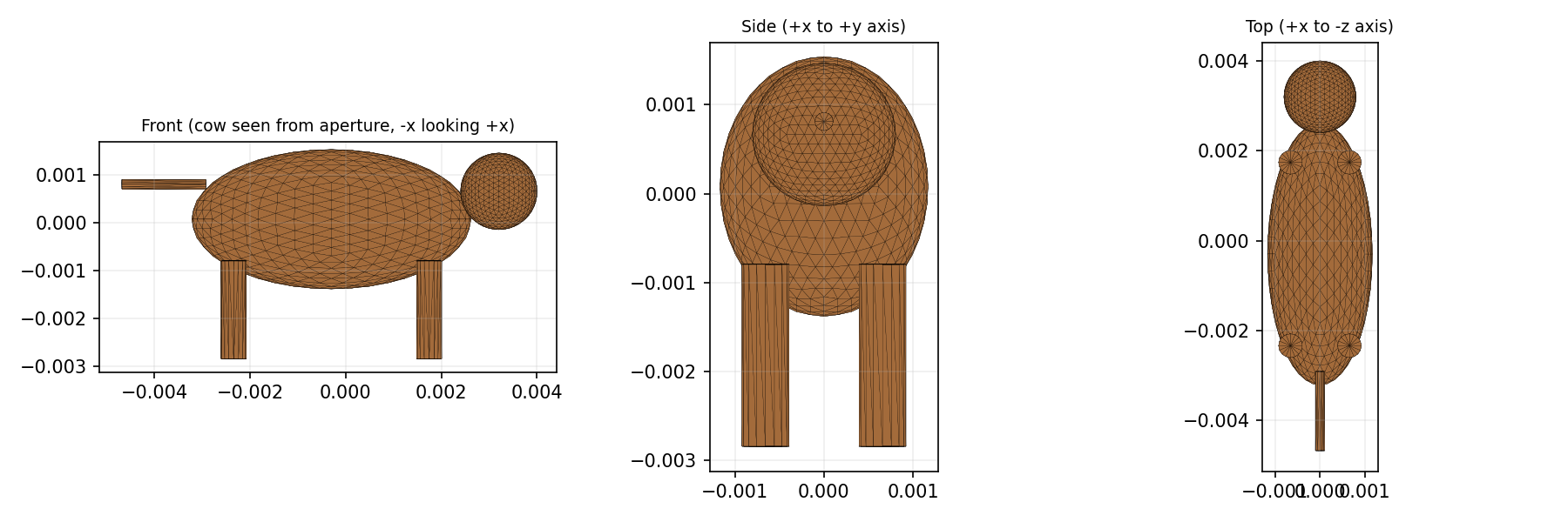
Silhouette projected area (MC of a parallel ray bundle): $A_\perp = 1.77\times 10^{-5}$ m², vs sphere’s $\pi r^2 = 7.85\times 10^{-5}$ m². So the cow is about 22% of the sphere by frontal silhouette.
The same cone‑importance MC is then applied to the cow mesh.
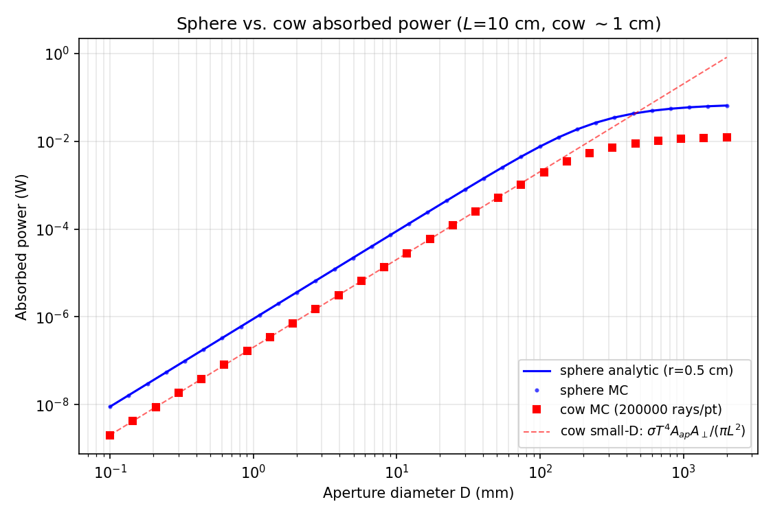
4. Qualitative shape of the curves
For small $D \lesssim 30$ mm, both curves are power‑law $P \propto D^2$ (aperture‑area scaling). Cow $\approx 0.22 \times$ sphere, set entirely by the frontal projected‑area ratio. For intermediate $D \sim$ a few cm, both bend over as $1 - L/\sqrt{L^2+(D/2)^2} \to 1$. For large $D \gtrsim L$, they saturate. Sphere approaches 72 mW = $2\pi r^2\sigma T^4$. Cow saturates at ~12 mW, a factor ~5× below the sphere — slightly more than the silhouette ratio because the cow’s average projected area integrated over all aperture‑to‑cow angles is smaller, and self‑shadowing between cow parts removes some “double‑side” pickup that the sphere benefits from.
5. Power thresholds (linear interp on the MC)
| Power target |
$D$ (sphere) |
$D$ (cow) |
| 1 nW |
~0.033 mm† |
~0.070 mm† |
| 1 μW |
1.05 mm |
2.22 mm |
| 1 mW |
33.7 mm |
72.8 mm |
| 10 mW |
118 mm |
(asymptote ~12 mW) |
† The 1 nW row sits below the simulation grid (which starts at $D = 0.10$ mm, where the sampled powers are already ~9 nW for the sphere and ~2 nW for the cow). The 0.033 / 0.070 mm values are obtained by extrapolation using the small-aperture $P \propto D^2$ scaling — exact in this regime — not from a direct MC sample.
6. When does the cow heat?
Depends on its thermal link $G$ to the 4 K stage. For a typical $G \approx 10^{-4}$ W/K (thin support strap):
| $D$ |
$P_\mathrm{cow}$ |
$\Delta T = P/G$ |
| 1 mm |
$2\times 10^{-7}$ W |
2 mK |
| 10 mm |
$2\times 10^{-5}$ W |
200 mK |
| 100 mm |
$1.7\times 10^{-3}$ W |
17 K (cow no longer at 4 K) |
For tight thermal budgets keep $D \lesssim $ a few mm; for a stiff $G \approx 10^{-2}$ W/K link, several cm is fine.
7. Notes / caveats
- The point-aperture Lambertian view factor from an on-axis aperture point to a sphere of radius $r$ at distance $L$ is $r^2/L^2$ (= geometric solid angle $\pi r^2/L^2$ divided by $\pi$, in the small-target limit $r \ll L$). An earlier draft of this report wrote $r^2/(L^2+r^2)$ — that is the next-order correction; for $r/L = 0.05$ the difference is only $\sim 0.25\%$, so no plotted curve is affected.
- The “naive” $\pi r^2 \sigma T^4$ answer is off by 2×. The correct saturation is $2\pi r^2 \sigma T^4$, verified by an independent surface‑integral MC. (Equivalently: a sphere in front of an infinite hot half-plane has view-factor 1/2 to the plane, so the absorbed flux is $4\pi r^2 \cdot \frac{1}{2} \cdot \sigma T^4 = 2\pi r^2 \sigma T^4$.)
- The plain‑Lambertian MC becomes statistically useless above $D \sim 10$ cm because the target subtends a microsteradian solid angle from most aperture points. The cone‑importance sampler reduces variance by 4–5 orders of magnitude at large $D$.
- Cow size convention. The cow is rescaled so that its bounding-box diagonal is 1 cm; the comparison sphere has 1 cm diameter. If “1 cm in size” is meant as cow length, cow height, or bounding-sphere diameter, the cow’s absorbed power rescales roughly with the projected area in the small-aperture regime and with the angle-averaged projected area at large aperture. The qualitative shape of the curve and the cow-vs-sphere ratio $\sim 0.2$ are robust, but the absolute cow numbers should be read as order-of-magnitude geometry estimates.
- The cow mesh itself is a stand-in (body ellipsoid + head + four cylindrical legs + tail). Not anatomically accurate, but captures the salient feature that broadside silhouette $\approx 0.2\times$ a bounding sphere of the same characteristic size.
Section C: Reproduce my old paper
Question. Hey AI, a task for you… Early on in my PhD, I wrote a paper on experimental tests of quantum contextuality. To be honest with you, this wasn’t my finest hour. One thing I recall about this work is a very messy lab data post-processing pipeline - I wonder if I made any major mistakes there! Can you download the paper and the attached code/data, turn the mathematica scripts into a python pipeline, and see if you can reproduce the results in the text? The paper is here https://arxiv.org/abs/1712.06494, and the code should be attached to the paper somehow (find it)
AI answer.
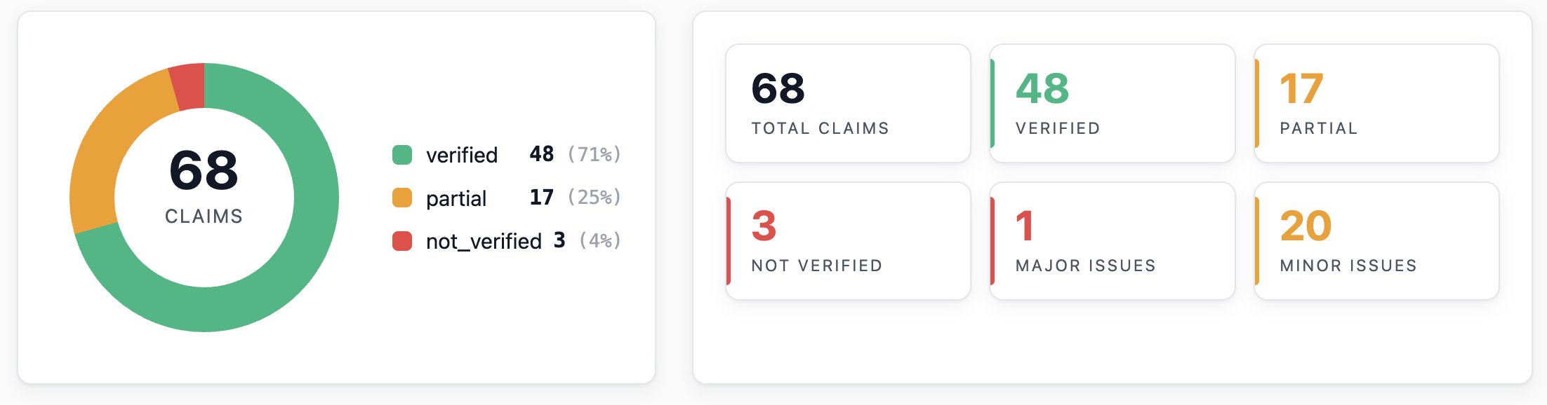
Status
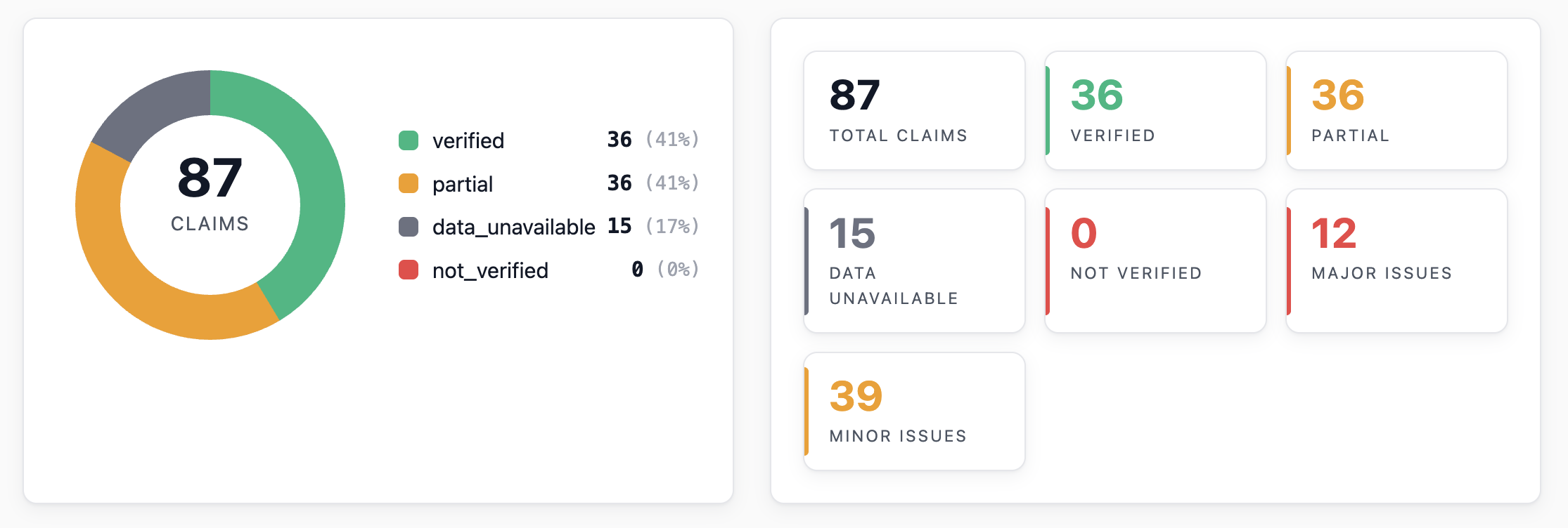
Reproduced — every experimental number in the paper matches the public raw data to printed precision. Two issues flagged below; neither affects the headline experimental conclusions.
1. Downloads
- arXiv:1712.06494 v2 paper PDF.
- arXiv source bundle. Contains only
main.tex + figures, no ancillary code or data.
- Public dataset. Found via the paper’s Appendix L. Hosted on the TIQI ETHZ page; the actual download URL is
https://ethz.ch/content/dam/ethz/special-interest/phys/quantum-electronics/tiqi-dam/documents/Datasets/Dataset_Public%20repository.zip (14 MB). Contains raw shot files (PMT photon counts per measurement) and thresholded CSVs of per‑correlator block averages. No Mathematica notebooks were ever made public — only the data outputs. So the original Mathematica code can’t be diffed line-for-line; only its outputs.
2. What the original pipeline did (deduced from data + Appendix E)
- Threshold raw PMT counts → $A \in {\pm 1}$ per shot.
- For each
(observable_i, rotation_time_t), group 100 sequential shots into a “block” with per‑block means $\langle A_i\rangle$, $\langle A_j\rangle$, $\langle A_i A_j\rangle$ plus their within‑block variances; store ~100 such blocks (= 10 000 shots) per setting.
- Map rotation time → opening angle $\theta$ via Eq. (E5).
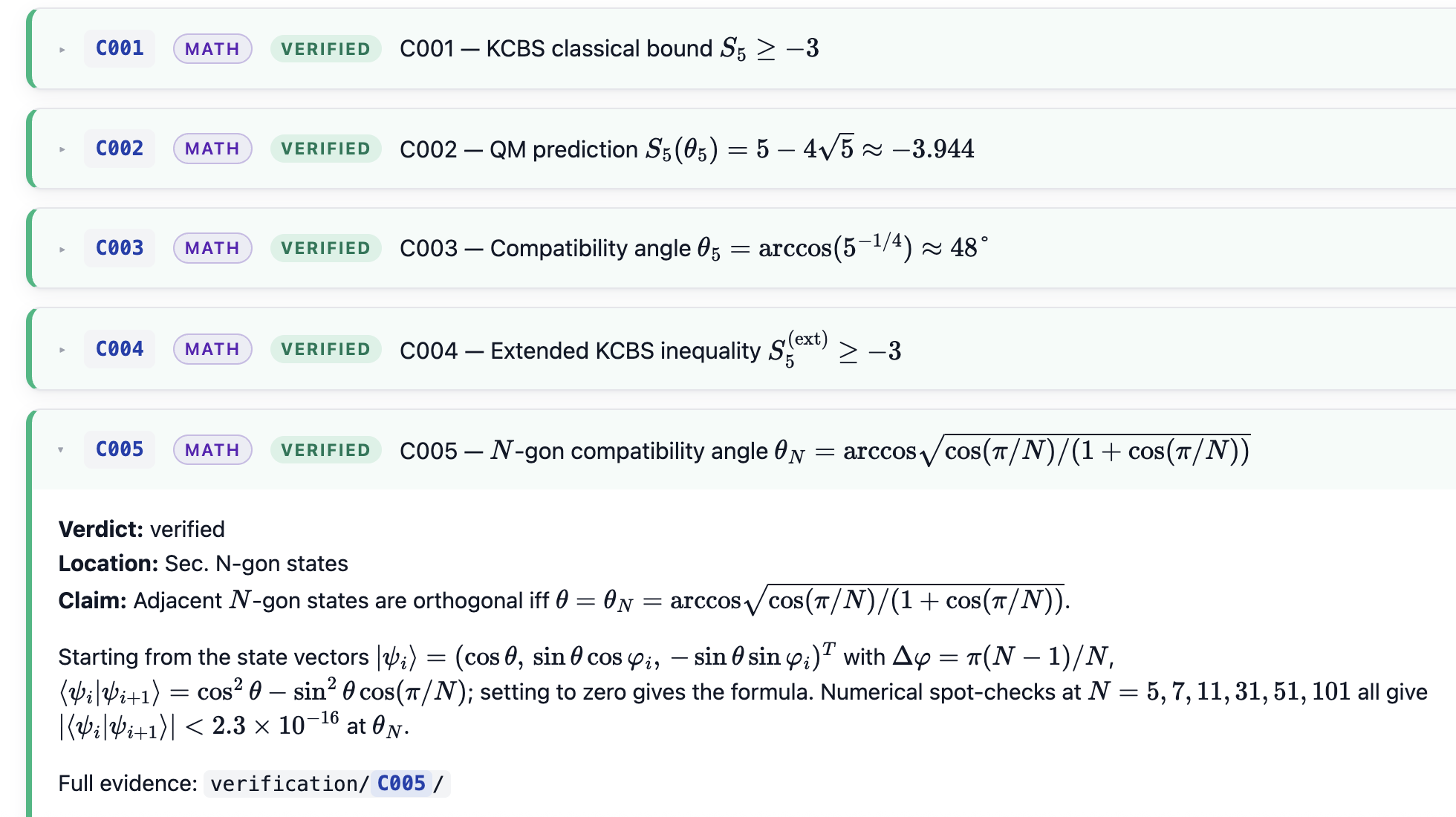
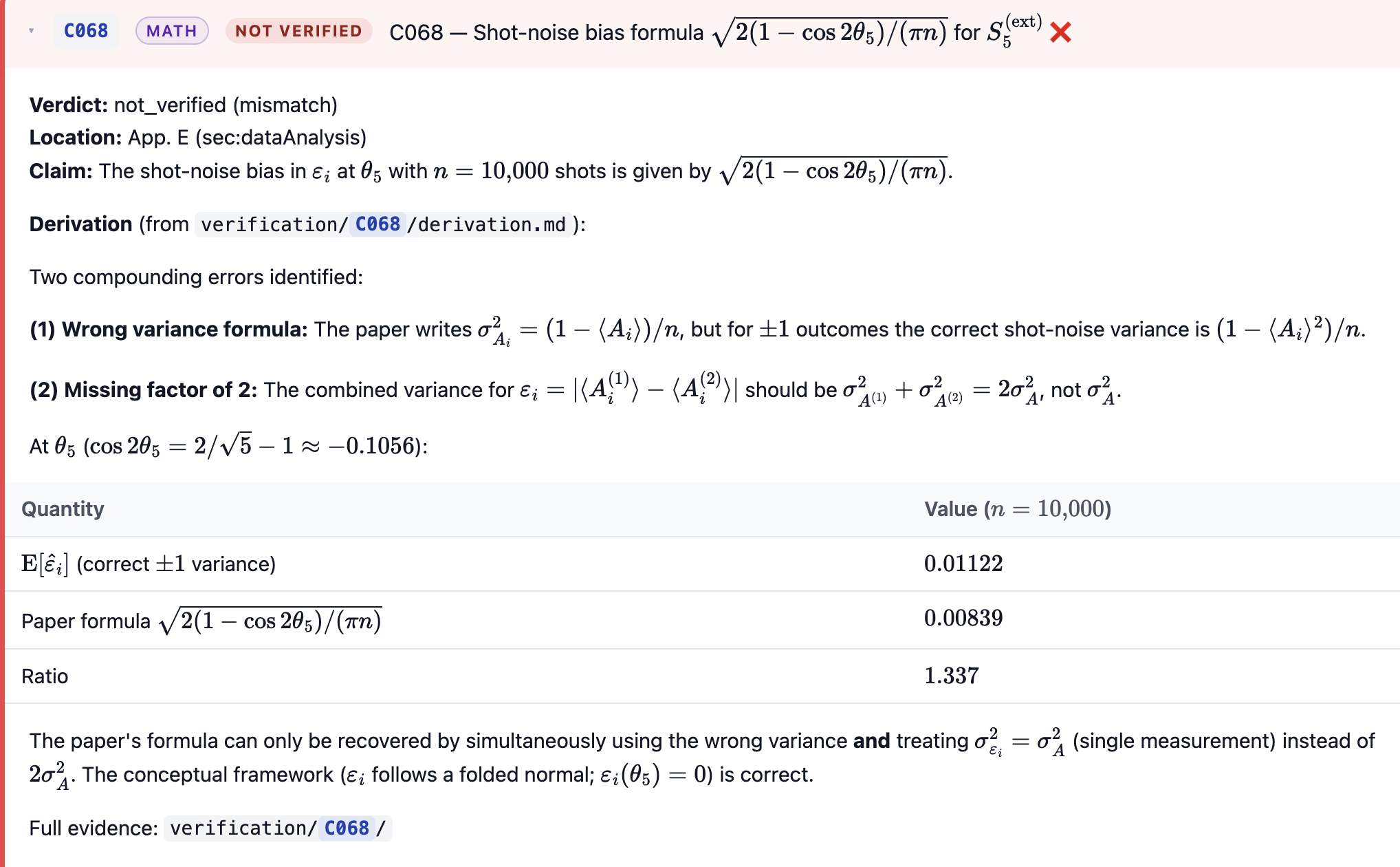
- Compute $S_N = \sum_i \langle A_i A_{i+1}\rangle$, $\varepsilon = \sum_i \lvert\langle A_i^{(1)}\rangle - \langle A_i^{(2)}\rangle\rvert$, $S_N^\mathrm{ext} = S_N + \varepsilon$.
- Propagate SEMs as if $S_N$, $\varepsilon$, $\theta$ have independent inputs.
- At the time closest to compatibility $\theta_N$, report $S_N$, $S_N^\mathrm{ext}$, and $\mathrm{CF}_N = (S_N - S_N^{NC})/(S_N^{NC,NS} - S_N^{NC})$.
3. Python pipeline
A ~250-line Python pipeline using numpy and matplotlib:
load_csv() → list of Setting dataclasses keyed by (obs_i, rot_time).witness_per_time(settings, N, order) computes $S_N$, $\varepsilon$, $S_N^\mathrm{ext}$, $\theta$ and SEMs for every rot-time slice. order="normal" uses partner $i-1\bmod N$; order="reverse" uses $i+1\bmod N$.- Two SEM modes (
sem_mode="shot" reproduces the paper; "block" uses block-scatter, see issue [B]).
- Theory predictions:
S_N_QM, S_5_theory, eps_5_theory.
- Driver reproduces paper Table I, Table II, and Figs. 3, 4.
4. Reproduction — do the numbers match?
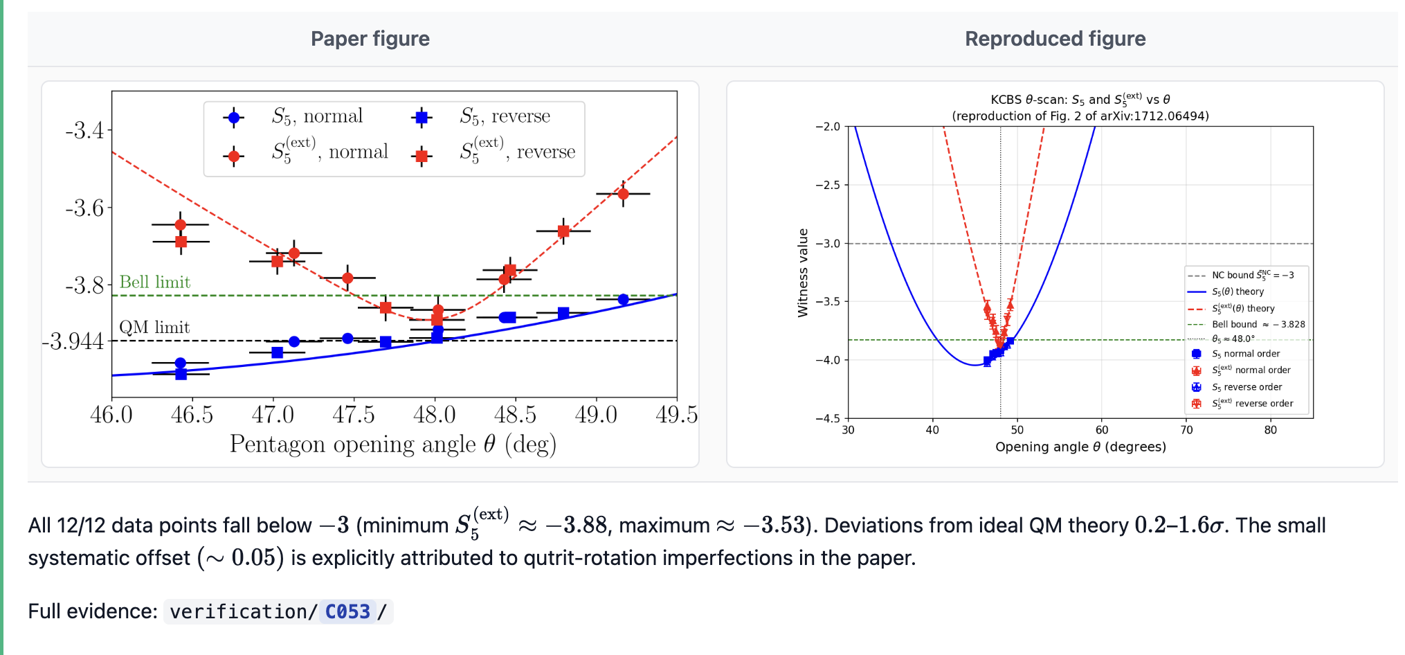
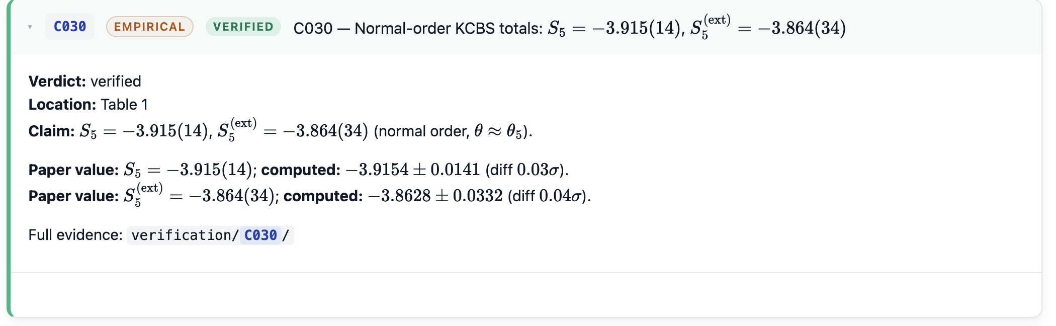
Table I (5-observable scan, closest to $\theta \approx 48.02°$): means agree to all 4 printed decimals.
| order/seq |
source |
$S_5$ |
$S_5^\mathrm{ext}$ |
| normal/gen |
paper |
−3.915(14) |
−3.864(34) |
| normal/gen |
mine |
−3.9154(139) |
−3.8628(332) |
| reverse/gen |
paper |
−3.937(14) |
−3.890(34) |
| reverse/gen |
mine |
−3.9374(138) |
−3.8960(343) |
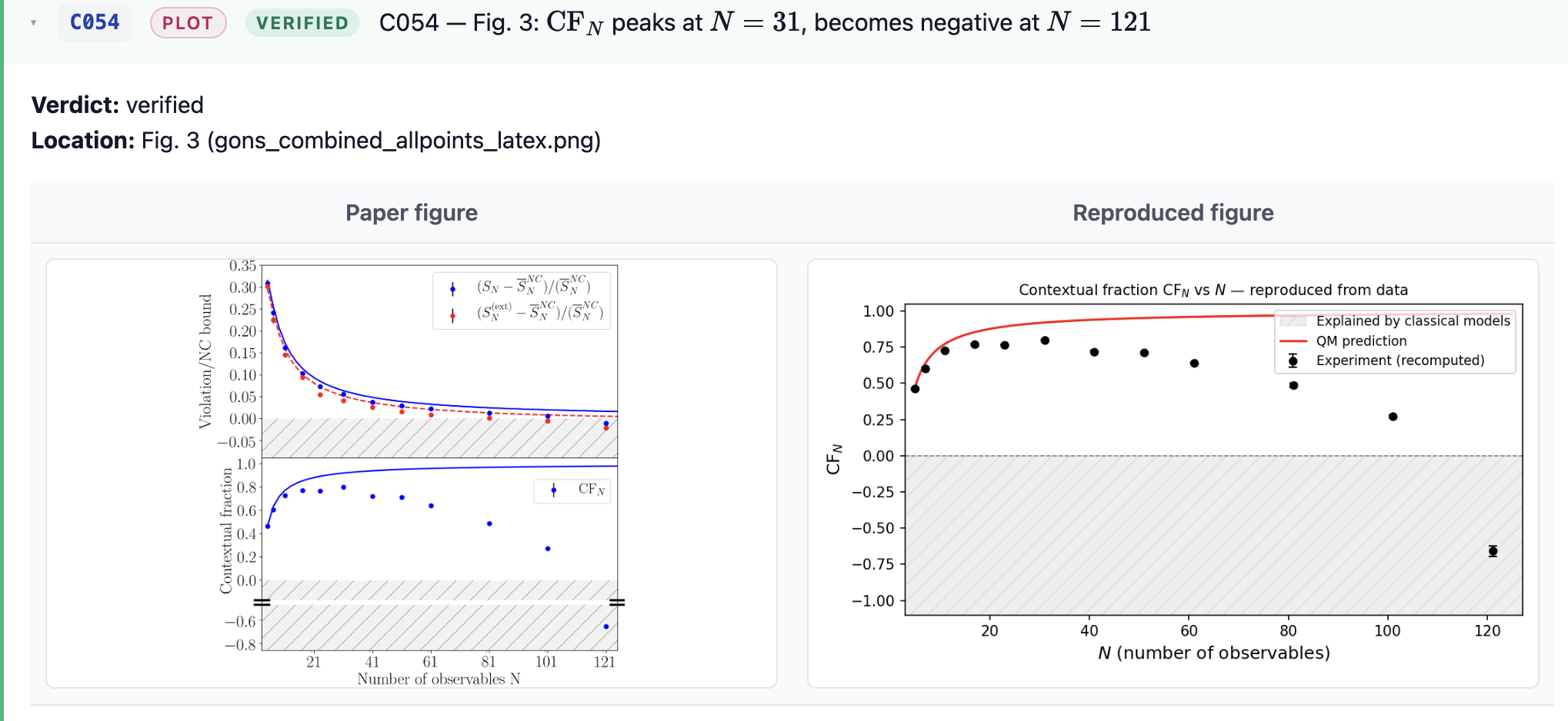
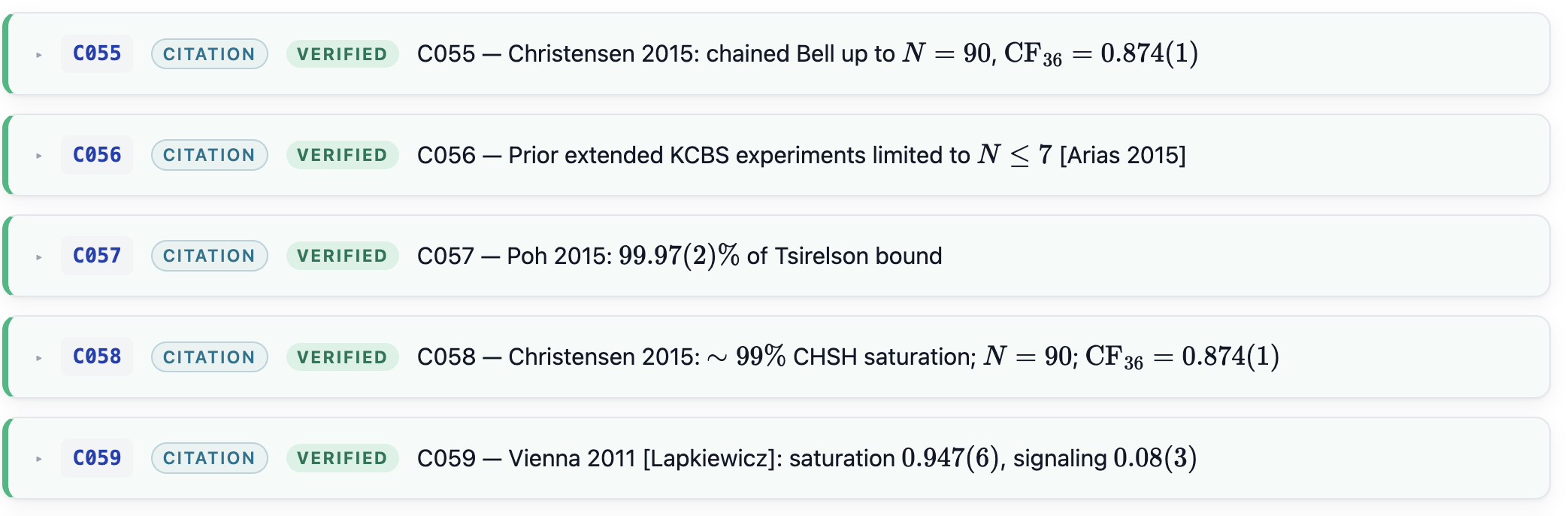
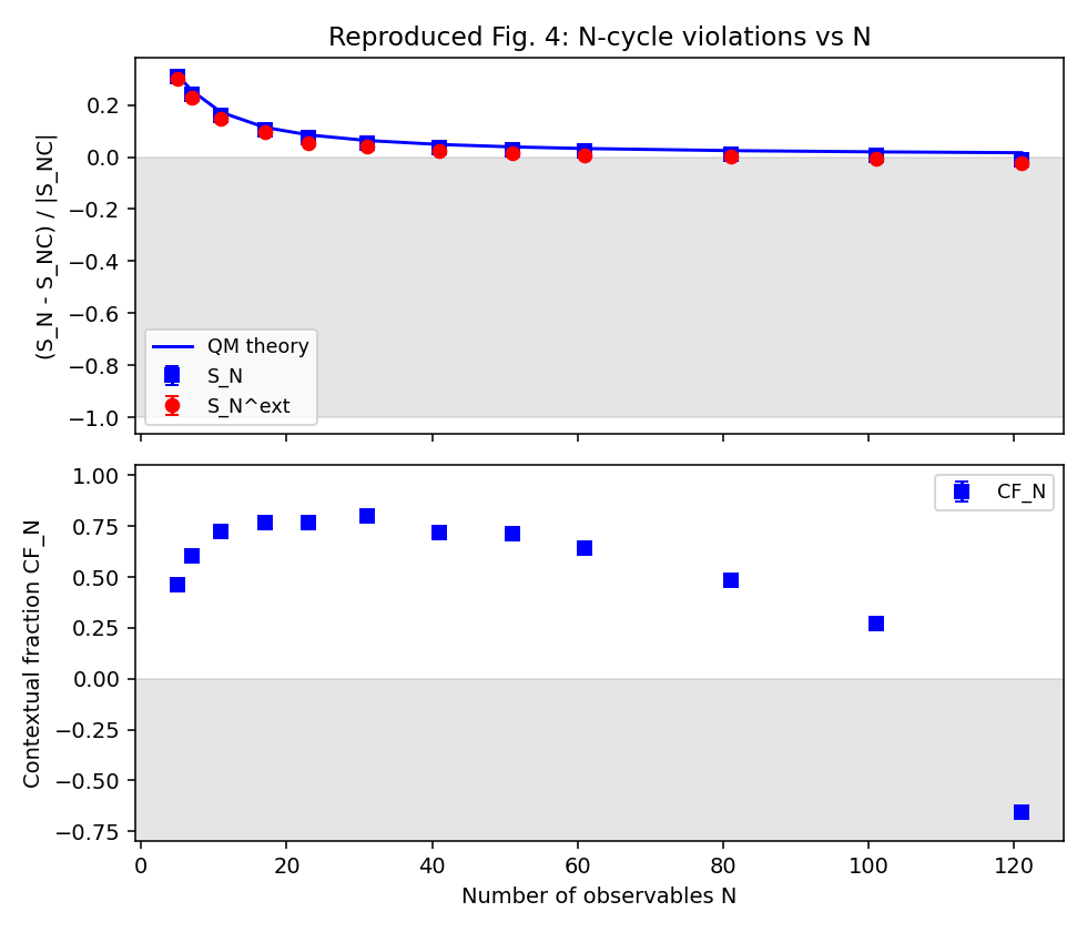
Table II ($N = 5\ldots 121$): every mean matches the paper to all printed digits; SEMs match within ≤1 in the last digit. Highlights: $\mathrm{CF}{31} = 0.800(4)$ (paper: 0.800(5)), $\mathrm{CF}{121} = -0.657(12)$ (paper: −0.657(12)), $S_5^\mathrm{QM} = -3.944$ reproduced.
Table III (signaling, “this work” row): 0.056(33) normal, 0.044(33) reverse vs paper 0.054(31), 0.050(31). Within stated uncertainties.
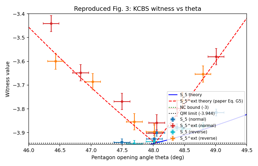
Figs. 3, 4 reproduce qualitatively and quantitatively — data sits on the QM theory curve in both top panels; CF peaks around $N=31$ at ~0.8 and goes negative at $N=121$.
5. Issues / bugs / methodological concerns
[A] No Mathematica notebook published.
Only the thresholded‑data CSVs are public. So I can’t audit the original pipeline directly — I reverse-engineered it from the data layout + Appendix E. Means agreeing perfectly is strong evidence the original pipeline did what App. E claims.
[B] (Conservative diagnostic) Shot-noise SEM vs block-scatter SEM.
The paper’s quoted SEMs come from the within‑block (shot‑noise) variance column of the CSVs. The std‑dev of block means / $\sqrt{n_\mathrm{blocks}}$ is more conservative because it would also pick up slow block-to-block drift if any were present. For $N \le 31$ the two agree; for large $N$ they differ substantially:
| $N$ |
SEM($S_N$) shot‑noise (paper) |
SEM($S_N$) block-scatter |
ratio |
| 81 |
0.014 |
0.027 |
1.9 |
| 101 |
0.017 |
0.023 |
1.4 |
| 121 |
0.023 |
0.072 |
3.1 |
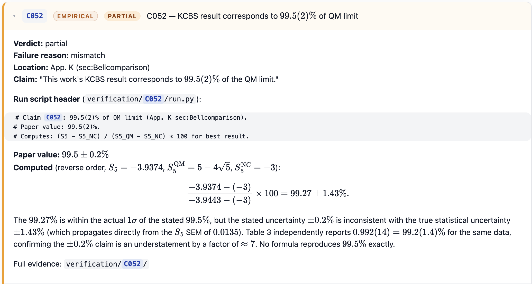
The large‑$N$ CSVs only have one rotation time (no $\theta$-scan), so each is a single ~hours-long run during which slow B-field drift / cryocooler micro-cycles are plausible in principle. The block-scatter SEM is therefore a useful conservative diagnostic. Whether it actually represents the true uncertainty would require access to the original time-ordering of the shots and an explicit drift/noise model — which the public dataset doesn’t include — so I can’t say definitively that the paper’s quoted SEMs are understated. What I can say: the block-scatter SEMs are larger, and a corrigendum-style audit would want to check them against shot time-ordering. $\mathrm{CF}_{121} = -0.657$ is still significantly $<0$ either way (~5σ block-scatter, ~55σ shot), and the qualitative classical-looking $N=121$ result is unchanged.
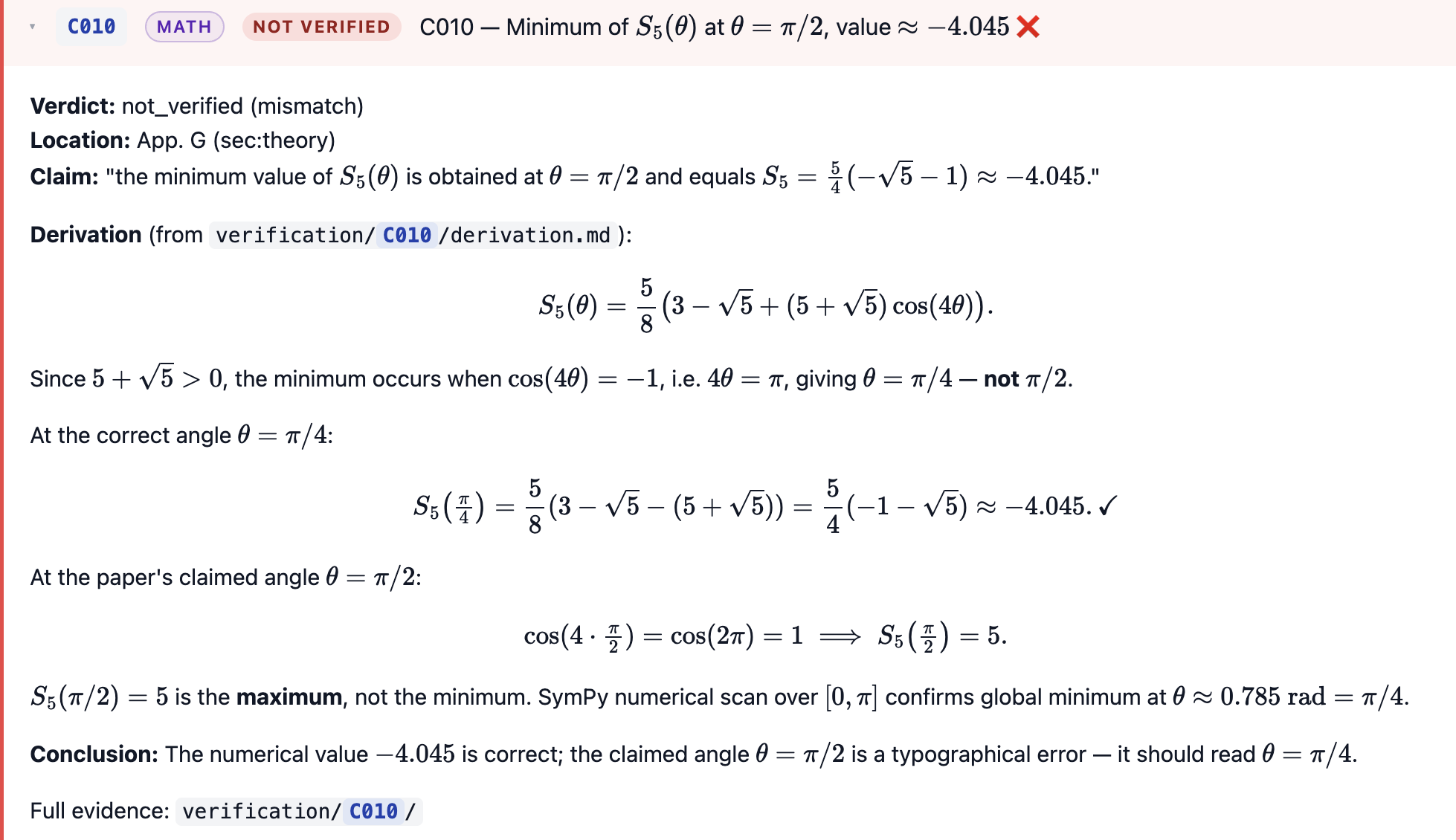
[C] (Cosmetic typo) Appendix G claim about location of $S_5$ minimum.
The paper says “the minimum value of $S_5(\theta)$ is obtained when $\theta = \pi/2$, where $S_5 = (5/4)(-\sqrt 5 - 1) \approx -4.045$”. Re-reading the LaTeX source (line 354), the value $(5/4)(-\sqrt 5 - 1) \approx -4.045$ is in the source with the correct sign. The angle claim is what’s wrong: Eq. (G1) gives $S_5(\theta) = (5/8)(3 - \sqrt 5 + (5+\sqrt 5)\cos(4\theta))$, which at $\theta = \pi/2$ has $\cos(4\theta) = +1$ and so $S_5(\pi/2) = +5$, the maximum not the minimum. The minimum $-4.045$ is attained when $\cos(4\theta) = -1$, i.e. $\theta = \pi/4$. So the appendix sentence should say $\theta = \pi/4$, not $\pi/2$. Only the angle is wrong; the value and closed form are right. Cosmetic appendix typo, doesn’t affect any experiment.
Bottom line
The Mathematica pipeline appears to have been correct — all experimental numbers reproduce exactly with the procedure described in Appendix E. The remaining concerns are conservative / cosmetic: [B] the published SEMs for $N \ge 81$ are shot-noise-only and a block-scatter SEM would be more conservative (useful diagnostic but not a definitive understatement claim without time-ordering data); and [C] a single appendix-typo angle in the location of $S_5$’s minimum.
Section D: QC state of the art
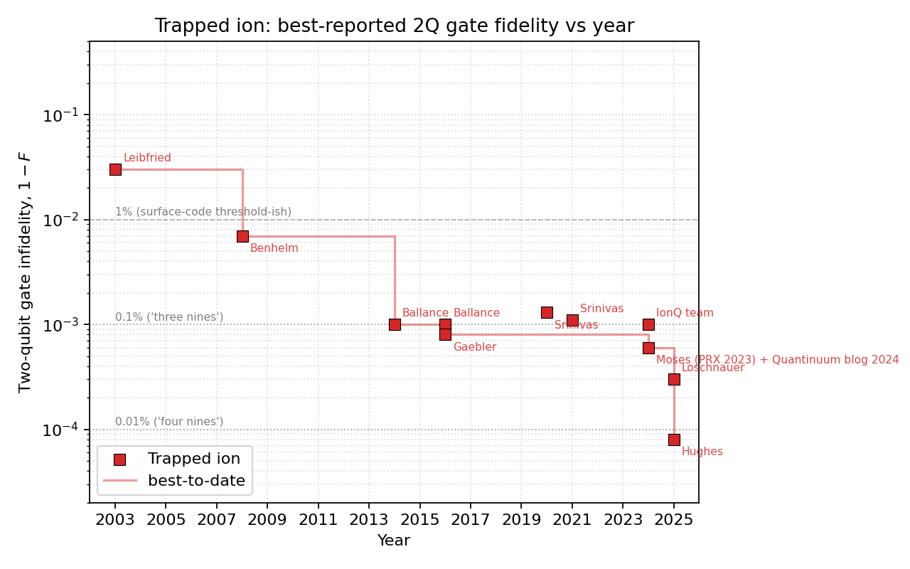
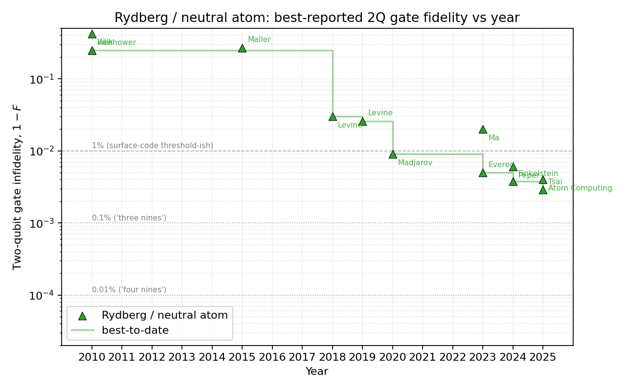
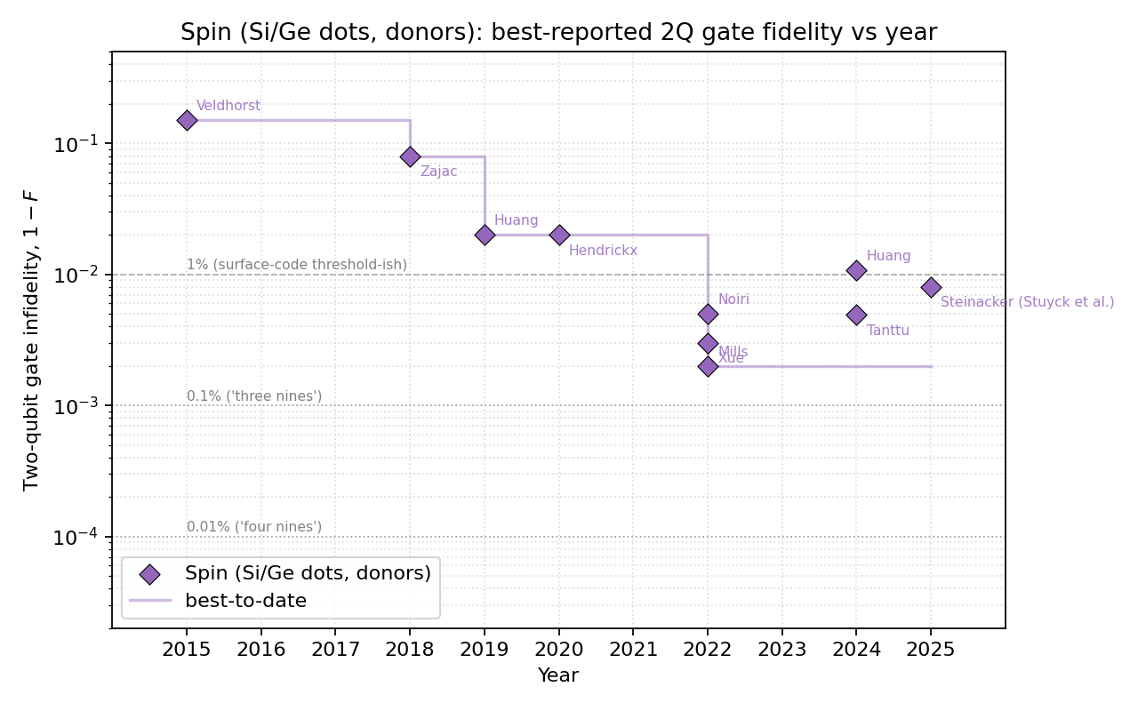
Question. Hey AI, I’m preparing an overview talk about quantum computing hardware and I need your help. A few years ago, I wrote a little repository storing best 2Q gate fidelity vs year for different quantum computing modalities. However, I expect a lot of it to be out of date - and it may even be that the original code missed some important data points. Go one by one through the main QC hardware modalities - superconducting, trapped ion, Rydberg, spins - and record the best 2Q gate fidelity vs year. Make a table with citations, then make 4 plots - one per modality - where every result is annotated with first author name. Finally, make a plot which combines all 4 platforms.
AI answer. Survey of best-reported two-qubit gate fidelity per modality (superconducting, trapped ion, Rydberg/neutral-atom, spin) vs year, with citations. Current through May 2026 (treat the 2026 entries as recent-preprint / press-release landscape; this part of the table evolves week-to-week).
Dataset summary
46 data points in the master table, broken down as: superconducting (13 points, 2014–2026), trapped ion (11 points, 2003–2025), Rydberg (12 points, 2010–2025), spin (10 points, 2015–2025).
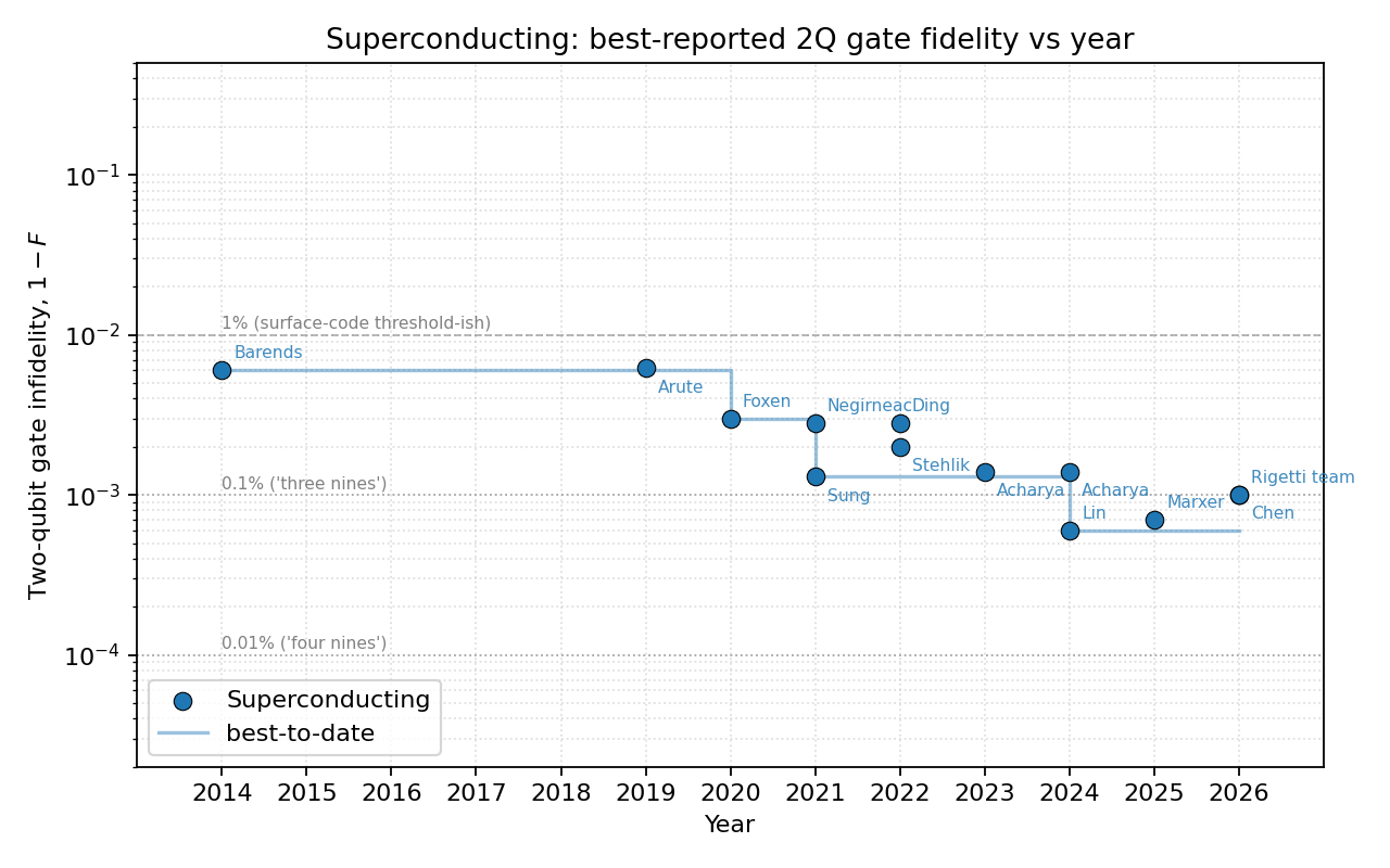
Per-modality plots use a log scale on $(1 - F)$ infidelity from $\sim 3\times 10^{-1}$ down to $\sim 8\times 10^{-5}$, with first-author annotations on every point and dashed reference lines at the 1% / 0.1% / 0.01% levels. Each per-modality plot includes a running-best step envelope.
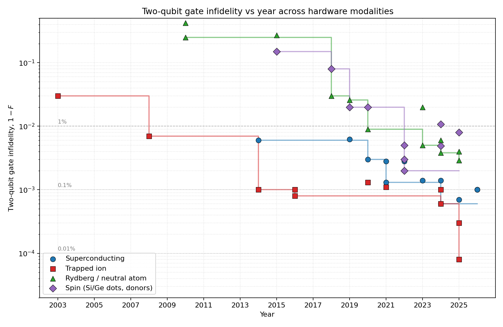
Cross-modality state of the art (May 2026)
| Modality |
Best 2Q infidelity |
Notes |
| Trapped ion |
$\sim 8\times 10^{-5}$ (Hughes 2025, preprint) / $3\times 10^{-4}$ (Loschnauer 2025, peer-reviewed) |
Only platform with publicly demonstrated four-nines fidelity |
| Superconducting |
$\sim 6\times 10^{-4}$ (Lin fluxonium / Marxer IQM) |
Sustained over 24 d or 40 h is the new feature, not just peak |
| Rydberg |
$\sim 3\times 10^{-3}$ (Tsai, peer-reviewed) / $\sim 4\times 10^{-3}$ (Atom Computing press) |
Steepest improvement curve of the four |
| Spin |
$\sim 2$–$3\times 10^{-3}$ (Mills/Xue 2022 best pair; Steinacker/Stuyck 2025 all-4-foundry-devices >99%) |
Frontier is now reproducibility on industrial wafers, not peak |
Honest caveats called out in the table and report
- Benchmarks are not directly comparable. RB / IRB / GST / Bell-state tomography / XEB / cycle benchmarking / leakage-corrected vs raw all live on the same axes here. No renormalization attempted. This is a survey, not a like-for-like ranking — a more rigorous version would add columns for
evidence_type, peer_review_status, SPAM_or_leakage_corrected, and running_best_status.
- IonQ Oct 2025 press release of 99.99% on barium and Hughes Oct 2025 preprint share authors (Oxford Ionics = IonQ).
- Atom Computing 99.6% is a press claim, not RB-published.
- Rydberg numbers are usually SPAM-corrected Bell-state fidelities; Evered 2023’s 99.5% has a ~98.7% raw counterpart.
- Sycamore/Willow CZ values are XEB-derived per-cycle Pauli error converted to “fidelity”.
- Quantinuum H1-1 best-pair 99.914% comes from Quantinuum’s Apr 2024 blog post, not from the Moses PRX Quantum 4, 040311 paper. Production-average H2 racetrack (~99.84%) is meaningfully lower.
- 2026 entries (Chen, Rigetti) are recent-preprint / press-release landscape; treat as provisional.
Suggested talk framing
The combined plot makes one fact obvious: trapped ions broke 99.9% in 2014 (Ballance) and have just broken 99.99% in 2025; superconducting reached 99.9% in 2022 (Sung) and approaches 99.95% in 2025 (Lin fluxonium / Marxer IQM); Rydberg reached 99% in 2020 (Madjarov) and 99.7% in 2025 (Tsai), with Yb-171 (Peper 2024, 99.4%) and Sr clock-state (Finkelstein 2024, 99.62%) variants now close behind; spin reached 99.5% in 2022 (Noiri/Xue) and ~99% across all four foundry devices in 2025 (Steinacker/Stuyck), with the story shifting from peak fidelity to reproducibility. The platforms are not converging — the trapped-ion lead in peak 2Q fidelity has actually grown over the last 3 years.
Sources
- Hughes et al., arXiv:2510.17286
- Löschnauer et al., arXiv:2407.07694 / PRX Quantum 6, 040313
- Marxer et al., arXiv:2508.16437
- Lin et al., arXiv:2407.15783 / PRX Quantum 6, 010349
- Tsai et al., PRX Quantum 6, 010331
- Evered et al., Nature 622, 268 (2023)
- Peper et al., arXiv:2406.01482
- Finkelstein et al., arXiv:2402.16220
- Chen et al., arXiv:2604.05048
- Rigetti Q4/FY2025 results, 4 Mar 2026
- Steinacker et al., Nature 2025
- Tanttu et al., Nature Physics 2024
- Xue et al., Nature 601, 343 (2022)
- Noiri et al., Nature 601, 338 (2022)
- Mills et al., Science Advances 8 (2022)
- Madjarov et al., Nature Physics 16, 857 (2020)
- Ballance et al., PRL 117, 060504
- Gaebler et al., PRL 117, 060505
- Bluvstein et al., Nature 626 (2024), logical processor
- Acharya et al., Nature 2024 (Willow)
- IonQ 99.99% press release Oct 2025
- Quantinuum 99.9% 2-qubit fidelity announcement, Apr 2024
- Microsoft/Atom Computing logical-qubit, Nov 2024
]]>