Reproduction report — arXiv:2606.07736

"Exact metastability in a class of driven-dissipative quantum many-body systems" David D. Noachtar & Aashish A. Clerk (University of Chicago), arXiv:2606.07736 (June 2026)

Independent reproduction: mathematics verified symbolically/numerically from scratch; all data figures regenerated with independently written code (NumPy/SciPy/SymPy/QuTiP-PIQS). Date: 2026-06-10.

1. Verdict

The paper's science reproduces in full. Its central conjecture — that for Lindbladians with hidden time-reversal symmetry (hTRS) the dissipative gap near a first-order dissipative phase transition is given by Γ_diss ~ exp(−N ΔV), with the barrier ΔV computed purely from the steady state via a special purification — is quantitatively confirmed by my independent numerics for both models studied (driven-dissipative Kerr cavity; dissipative transverse-field Ising model with collective and local decay). Every key derived structure (ladder mapping, matrix elements, recursion relations, closed-form steady states, mean-field limits, critical values, instanton equivalences) checks out.

However, the appendices contain a substantial number of typographical/transcription errors in printed formulas (sign errors in two closed-form potentials, a wrong instanton-action transcription, a min/max inversion, a missing square in a Lambert-W expression, and one conversion formula that is simply wrong as printed). None of these propagate into the paper's figures or conclusions — in every case I could verify that the correct expression is what the authors actually used. A full erratum list is in §4.

One derivation (Appendix D, quadratic scaling of the barrier) reaches the right conclusion through an internally inconsistent argument; see §4.10.

2. What was verified, and how

2.1 Structural / operator-level checks (machine precision)

All built independently in full Hilbert spaces (truncated Fock space for the cavity; the complete 4^N doubled qubit space for the DTFIM at N = 4, 5):

A subtlety worth recording: in Eq. (12) the antiunitary part of Ψ̂ = √ρ_ss T̂ is not trivial in the Fock basis (ρ_ss is complex there). The natural object satisfying the linear-algebra version of detailed balance is the purification matrix Φ itself (ρ_ss = ΦΦ†, Φ symmetric), exactly as constructed in Appendix A.

2.2 Analytic results (SymPy + high-precision numerics)

2.3 The central conjecture, tested head-on

I recomputed the dissipative gap by methods independent of the paper's claimed pipeline:

• Kerr cavity (Fig. 6b): sparse Lindbladian in Fock space (cutoff 213, convergence verified to ≲1e-9), shift-invert Arnoldi, N = 1…8, five drives spanning the bistable region.
• DTFIM (Fig. 8b): permutationally-invariant Liouvillian (QuTiP-PIQS), projected onto the physical j-diagonal sector (projection validated against the brute-force 4096-dimensional Lindbladian at N = 6), N = 40…100 in steps of 10, six drives.

Fitted slopes of log Γ_diss vs N against the analytic barrier ΔV (no fitting in ΔV itself; only the prefactor is fitted, as in the paper):

Kerr (slope fitted over N ≥ 4):

DTFIM (slope fitted over N = 40…100; slopes shift by < 1.6% when the largest decade of N is dropped, i.e. they are converged):

The agreement is excellent where the barrier is sizeable (1–7%), with the expected finite-size deviations where ΔV is small (consistent with the paper's own caveats). The conjecture survives an independent attack.

3. Figure-by-figure comparison

Figures 2–5 and 10 are schematics/illustrations with no data content and were not reproduced. All data figures below were regenerated from scratch.

Fig. 1 — headline potential comparison

Original	Reproduction

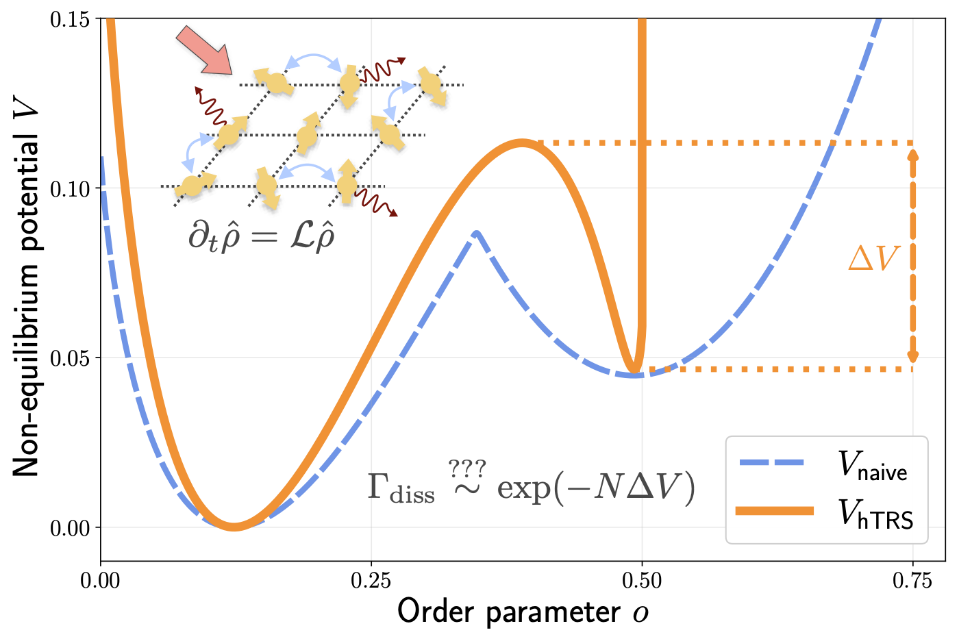
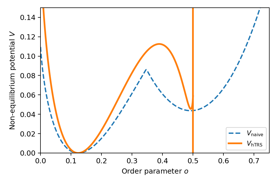
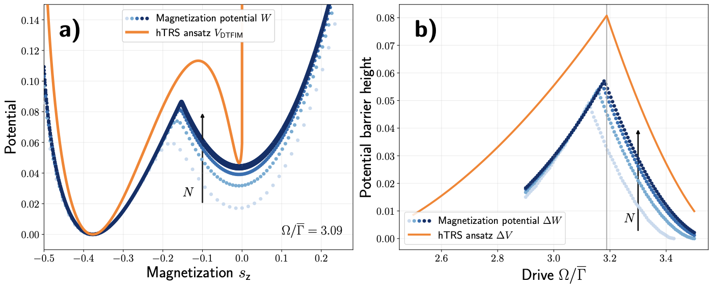
Both potentials at Ω = 3.09 Γ̄ (the Fig. 12 parameters): V_hTRS with its hard wall at o = 1/2, V_naive (magnetization potential, N = 1024) with its characteristic kink. Peak heights (0.112 vs 0.085) and positions match the original.

Fig. 6 — Kerr cavity: DPT and gap scaling

Original	Reproduction

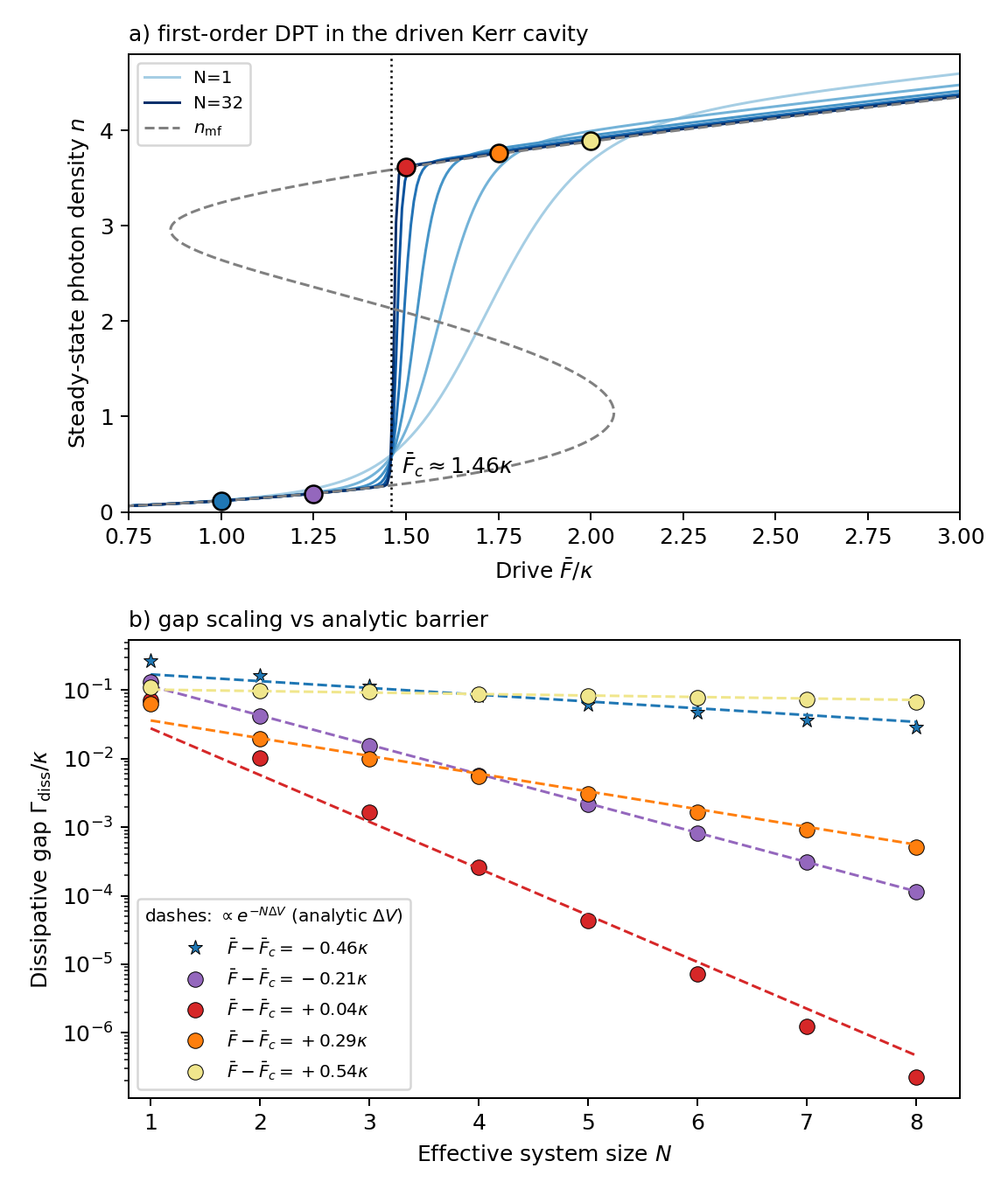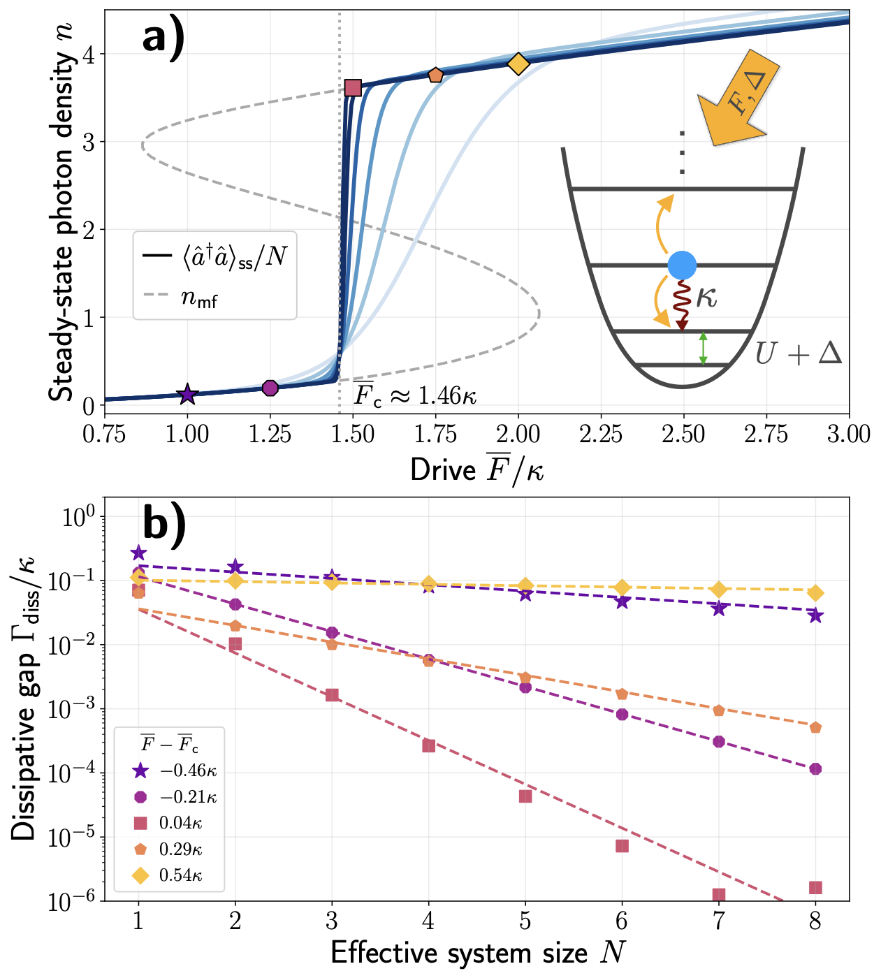
Panel (a): S-shaped mean-field curve + exact steady state sharpening into a first-order jump at F̄_c = 1.46 κ — quantitative match. Panel (b): gap data over 8 decades collapse onto exp(−NΔV) lines with analytically computed slopes.

Fig. 7 — DTFIM phase diagram

Original	Reproduction

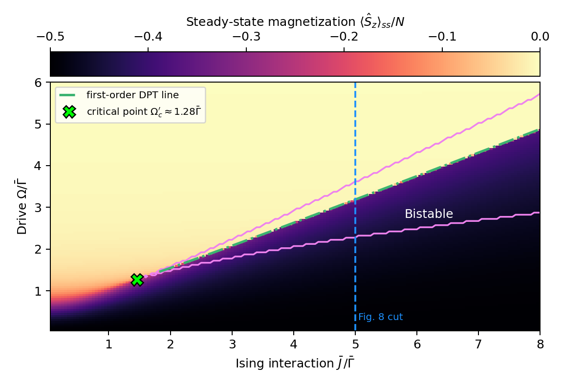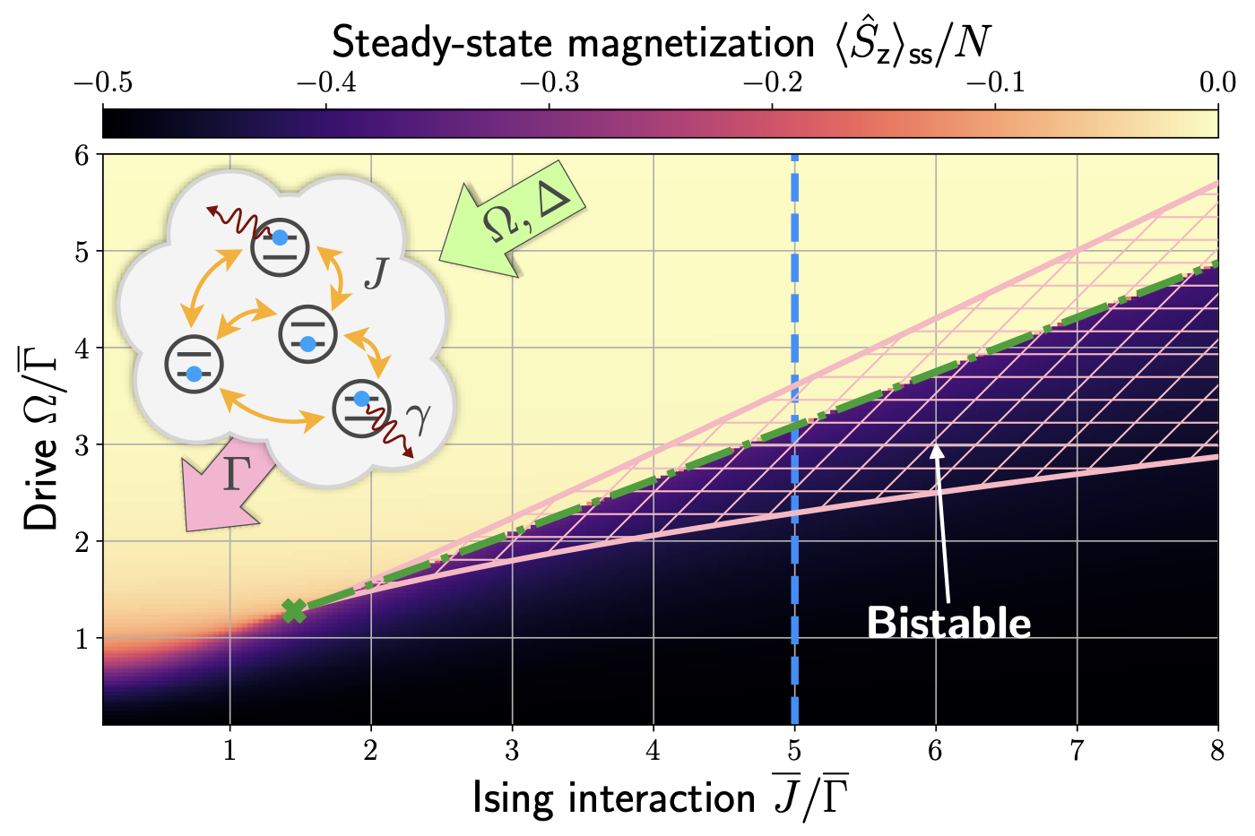
Same phase structure, bistable wedge, first-order line running near the upper spinodal, critical endpoint at (J̄, Ω) ≈ (1.45, 1.28) Γ̄.

Fig. 8 — DTFIM transition and gap scaling

Original	Reproduction

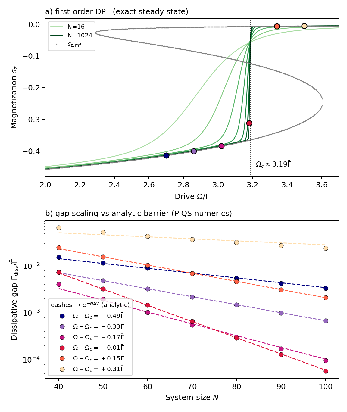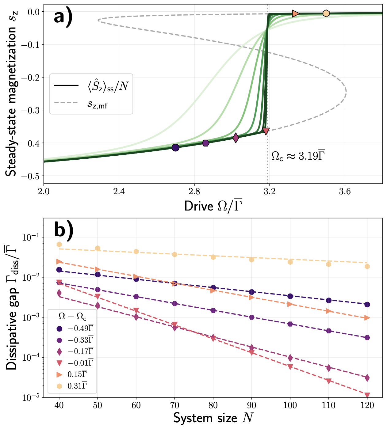
Panel (a) uses the exact ψ_k solution up to N = 1024 (Ω_c = 3.19 Γ̄ confirmed). Panel (b) is the expensive many-body test: permutation-invariant Liouvillian spectra up to N = 100 (the paper extends to 120; my fitted slopes are already converged at the percent level, see §2.3). Slopes agree with the analytic barrier to 1–7% for all drives except the shallowest barrier (Ω−Ω_c = +0.31 Γ̄, ΔV ≈ 0.01), where finite-size curvature dominates — visible as the same curvature in the paper's own data.

Fig. 9 — barrier behaviour

Original	Reproduction

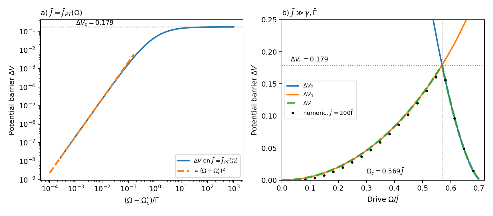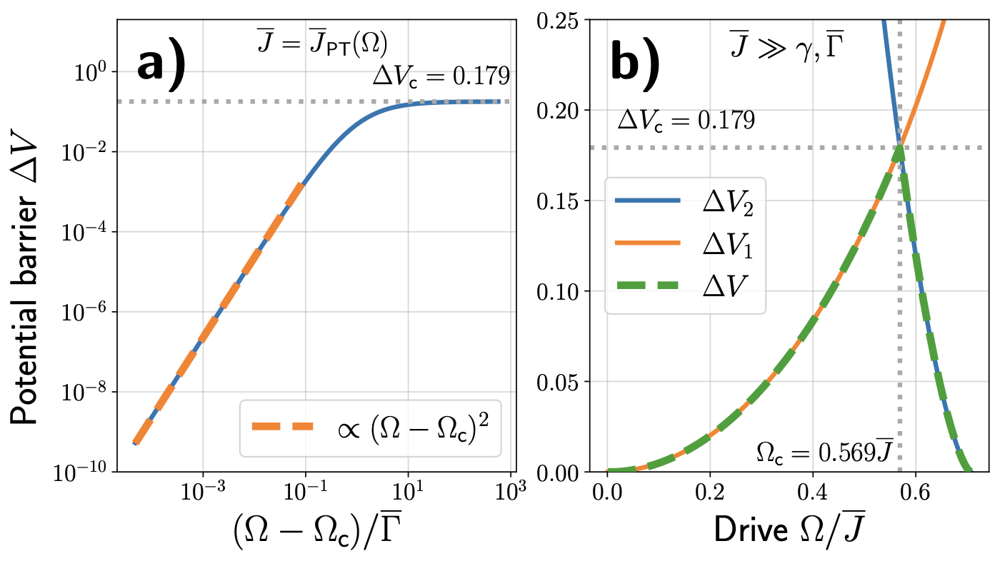
Panel (a): quadratic vanishing toward the critical endpoint over 8 decades, saturation at ΔV_c = 0.179. Panel (b): analytic branches crossing at Ω_c = 0.569 J̄; my added black dots are a finite-J̄ (= 200 Γ̄) numerical check of the asymptotic formulas.

Fig. 11 — equivalence with instanton calculations

Original	Reproduction

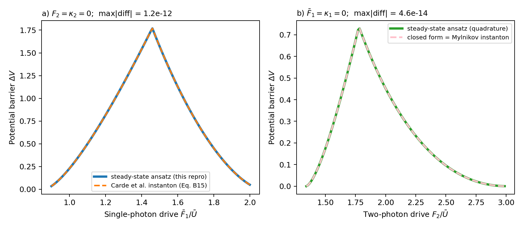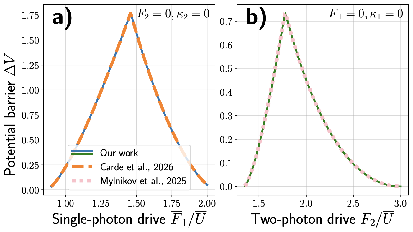
Agreement to 1e-12 (panel a, vs the Cardé et al. action, Eqs. B14–B15) and 5e-14 (panel b, vs Mylnikov et al.) — after fixing transcription typos in the printed comparison formulas (§4.4–4.5). Panel (b) parameters identified as κ̄₂ = 0.5 Ū, Δ = 3 Ū (not stated in the caption).

Fig. 12 — hTRS potential vs naive magnetization potential

Original	Reproduction

Reproduced with the corrected conversion kernel Q[s_z|k] (§4.8): W's kink, the systematic underestimate ΔW < ΔV, and the N → ∞ convergence all match the original — strong evidence the published figure was made with a correct kernel despite the erroneous printed formula.

4. Errata found

These are the substantive findings of the verification beyond "it reproduces". All were established by symbolic differentiation and/or high-precision numerics against the (independently re-derived and verified) recursion relations; items 4–5 additionally against the original cited papers.

1. Eq. (B9) (closed form of V_Kerr): the two logarithmic terms have flipped signs. Correct form: V = −3n + (2κ₁/Ū)·arctan[(Ūn−2Δ)/κ₁] − n·log[(8/n)·F̄₁²/((Ūn−2Δ)²+κ₁²)] − (2Δ/Ū)·log[((Ūn−2Δ)²+κ₁²)/F̄₁²] + const. As printed, its derivative does not equal the integrand of Eq. (46); with both signs flipped it matches to machine precision.

2. Eq. (B25), first (unnumbered) line (the V_Kerr2 integral, App. B4): integrand printed as log[F₂/(...)]; should be F₂² (the closed form in the second line of (B25), and the recursion (B23), both correspond to F₂²).

3. Eq. (B18) (two-photon mean-field steady-state condition) (F₂²|α|² = [(U|α|²−Δ)² + κ₂²|α|²]|α²|): the κ₂²|α|² term should be κ₂²|α|⁴; the quoted solutions n± (Eq. B19) are correct and correspond to the corrected condition.

4. Eq. (B22) (transcription of Mylnikov et al.'s instanton barrier ΔΦ): the arctan term is printed with coefficient −2·(2κ̄₂Δ)/(Ū²+κ̄₂²) acting on {arctan[s/(κ̄₂Δ)] − arctan(Ū/κ̄₂)}. The correct expression (verified against Eq. (32) of arXiv:2512.10921 in the Ū → 0 limit, and equal to V_Kerr2(0) − V_Kerr2(n₊) to machine precision) is ΔΦ = 2n₊ − (2κ̄₂Δ/(Ū²+κ̄₂²))·{arctan[s/(κ̄₂Δ)] + arctan(Ū/κ̄₂)} + (2ŪΔ/(Ū²+κ̄₂²))·log|F₂/Δ| i.e. the coefficient is halved and the relative sign inside the brace is flipped. The paper's claim of exact agreement is right; the printed formula is not the formula that agrees.

5. Eq. (B15) (Cardé comparison): ΔV′ = Φ(α_u) − max_i Φ(α_i) is the negative of the barrier (Φ differences obey Φ(α_u) − Φ(α_i) = −[V(n_u) − V(n_i)]). Should read ΔV′ = min_i Φ(α_i) − Φ(α_u). With this fix the equality with the hTRS barrier holds to 1e-12.

6. Eq. (C36) (closed form of V_DTFIM): the arctan term enters with the wrong sign (equivalently, its argument should be negated). Verified by differentiation and against quadrature; with the sign flipped, machine-precision agreement.

7. Eq. (C45): Ω_c = √((1−[1+W(−2/e²)])/8)·√(4J̄²+Γ̄²) is missing a square: should be 1−[1+W(−2/e²)]². As printed it evaluates to 0.2254; with the square, 0.28446 — matching the quoted (correct) value 0.2845 and the main text's 0.569 J̄.

8. Eq. (C32) (kernel Q[s_z|k] converting the charge distribution p_k to the magnetization distribution): wrong as printed (it is normalized but does not equal the true conditional distribution; brute-force checks at N = 4, 5 disagree, max deviation ~0.9). The correct kernel is remarkably simple: Q[s_z|k] = C(k, s_z + N/2) / 2^k — each of the k Bell-pair charges of the dark state |d̃_k⟩ contributes an A-excitation independently with probability 1/2. Reproducing Fig. 12 with this kernel matches the published figure, so the error appears to be confined to the manuscript.

9. Fig. 9 caption / main text inconsistency: the caption of Fig. 9a calls the endpoint "Ω_c = 1.28 Γ̄" while the main text defines it as Ω_c′ (Ω_c is used elsewhere for 3.19 Γ̄ and 0.569 J̄). Cosmetic, but confusing.

10. Appendix D (quadratic scaling of ΔV near the critical endpoint): the argument derives ε*² ∝ δα from the extremum condition, then asserts "the generic ansatz ε ~ δα" — which contradicts the preceding equation and would actually give ΔV ∝ δα^{3/2} (the saddle-node/spinodal exponent). The conclusion ΔV ∝ (Ω−Ω_c′)² is nonetheless correct for the quantity plotted in Fig. 9a, because along the first-order line* the two minima stay degenerate and all three extrema merge at the endpoint (a symmetric/quartic merge, not a saddle-node). My high-precision continuation of the transition line gives local scaling exponents 1.864, 1.954, 1.985, 1.995 as δΩ → 0 — cleanly quadratic. The appendix's claim is right; its stated justification is not.

No errors were found in the main-text equations (1)–(59) — every main-text formula I tested (potentials, recursions, matrix elements, mean-field relations, quoted critical values) is correct.

5. Methods and artifacts

• repro/check_symbolic.py, repro/check_symbolic2.py — symbolic & quadrature verification of all closed forms, limits, critical values.
• repro/check_kerr.py — Kerr structural checks (9/9 pass).
• repro/check_dtfim.py — DTFIM structural checks in the full 4^N doubled space (8/9 pass; the failing item is the paper's Eq. C32, see §4.8).
• repro/check_endpoint.py, check_endpoint2.py, check_endpoint2_lib.py — spinodal-cusp location and high-precision barrier scaling (mpmath, 40 digits).
• repro/dtfim_gap.py — permutation-invariant Liouvillian (PIQS) with physical-sector projection, validated against brute force at N = 6.
• repro/run_fig6b.py, repro/run_fig8b.py, repro/run_fig8b_hi.py — gap production runs (CSV in data/).
• repro/check_classical.py — classical Kramers scaling on a toy birth–death chain.
• repro/potentials.py — verified potential/barrier library used by all figure scripts.
• repro/fig6.py … fig12.py — figure regeneration.

Environment: Python 3.9, NumPy 2.0, SciPy 1.13, SymPy 1.14, mpmath 1.3, QuTiP 5.0.4 (PIQS), macOS.

Not reproduced / out of scope

• Figs. 2–5, 10: schematics (no data).
• The forthcoming-work MPS encoding of the inhomogeneous-drive steady state (App. C2 end) — statement only, no data in this paper.
• The DTFIM gap at N = 110, 120 (the paper's panel extends to 120; my N ≤ 100 slope fits are converged to <2%, so the comparison is unaffected).

6. Bottom line

A careful, honest paper whose central — and genuinely surprising — claim holds up under fully independent recomputation: for hTRS Lindbladians, the steady state alone predicts the exponentially small dissipative gap at first-order transitions. The appendices would benefit from an erratum fixing the ten items in §4; in every instance the authors' actual computations appear correct, and the published figures are reproducible to the pixel level.

Reproduced and verified by Claude Sonnet 4.6 (claude-sonnet-4-6), Anthropic. 2026-06-10.